1181
Technical Committee 106 /
Comité technique 106
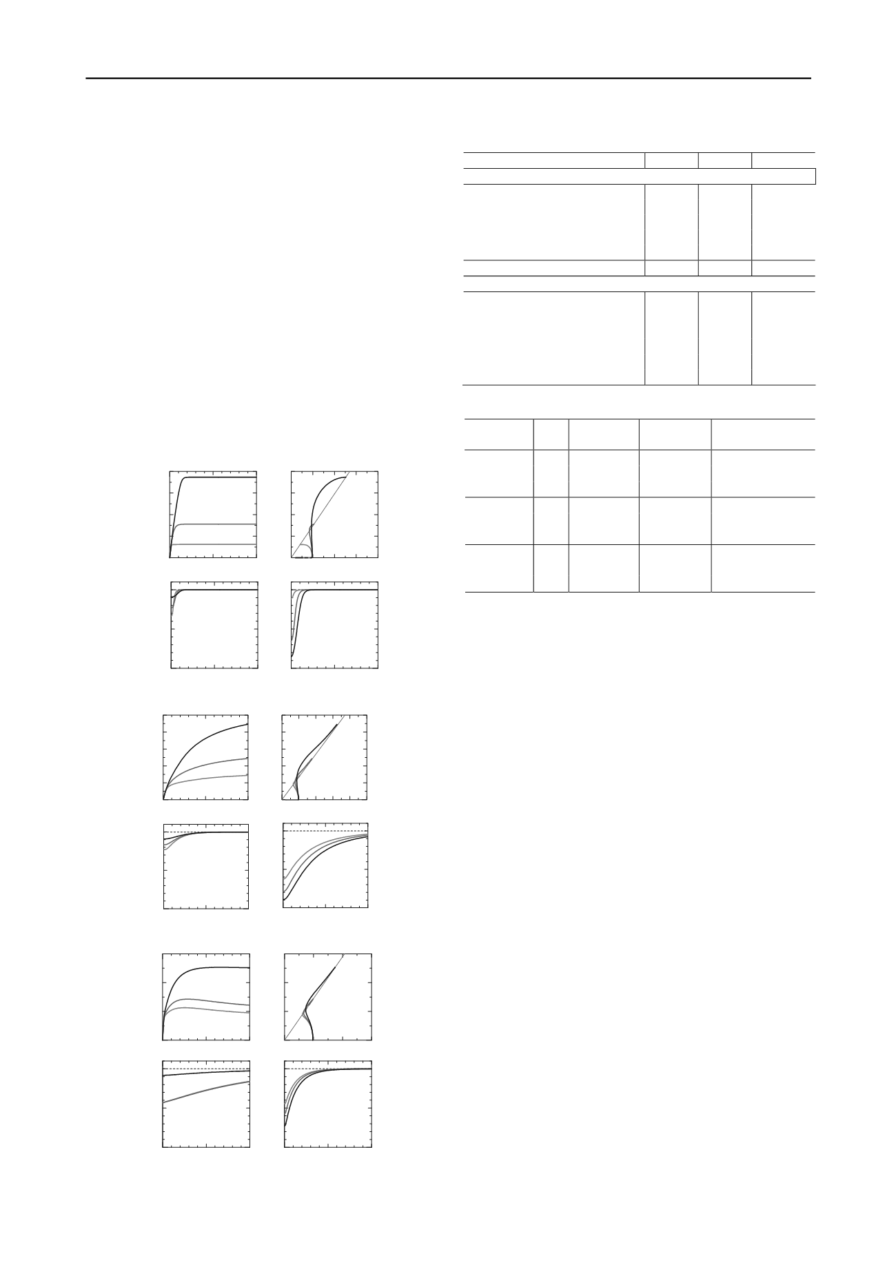
obtained in the compaction test, such as material A, the decay of
structure and loss of overconsolidation are fast. On the other
hand, in the case of materials for which a small maximum dry
density was obtained in the compaction test, such as material C,
there was little decay of structure, and loss of overconsolidation
was moderate. Finally, for material B, the results indicated that
the decay of structure was fast and that the loss of
overconsolidation was slow. As the maximum dry density
increased, decay of structure occurred faster. However, there
was no correlation between the rate of loss of overconsolidation
and the maximum dry density. Also, focusing on the initial
values, for all materials, it can be seen that as the Dc increased,
the structure decayed, and overconsolidation accumulated. Also,
it can be seen that for material such as C with small maximum
dry densities, structure and overconsolidation tend to remain
even though they are compacted. It can be inferred that this is
because there is little decay of structure due to shearing. Also,
focusing on materials A and B at Dc of 95–100%,
overconsolidation increases suddenly as a result of compaction.
At this time, the
q
also increases greatly. It can be seen that the
increase in
q
of compacted soil can be determined by the ease of
accumulation of overconsolidation.
Table 2 Material constants
Material
A
B
C
Elasto-plastic parameters
Compression index
0.07
0.11
0.13
Swelling index
0.01
0.02
0.01
Limit state index
1.48
1.35
1.45
NCL intercept (98.1 kPa)
1.50
1.71
2.07
Poisson’s ratio
0.30
0.30
0.30
Normal consolidation index
5.00
0.50
1.30
Evolution rule parameters
a
10.0
2.00
0.80
b
1.00
1.00
1.00
c
1.00
1.00
1.00
Structure decay index
s
c
1.00
1.00
0.40
Rotational hardening index
0.00
0.10
0.00
Rotational hardening limit constant
0.10
0.40
1.00
Table 3 Initial values
Material
Dc
Specific
volume
Extent of
structure Overconsolidation
90
1.55
1.50
3.77
95
1.47
1.30
13.2
A
100 1.40
1.10
32.0
90
1.72
1.30
8.10
95
1.64
1.20
19.1
B
100 1.56
1.10
42.5
90
2.17
2.20
5.1
95
2.08
1.90
9.8
C
100 1.98
1.40
16.2
0
10
20
200
400
0
200
400
200
400
Shear strain
s
(%)
Deviator stress
q
(kPa)
Mean effective stress
p
(kPa)
Deviator stress
q
(kPa)
q =
M
p
0
10
20
0.5
1.0
Shear strain
s
(%)
R*
Decay of structure
very fast
Loss of
overconsolidation
very fast
0
10
20
0.5
1.0
Shear strain
s
(%)
R
5 SEISMIC RESPONSE ANALYSIS OF EMBANKMENTS
Fig. 7 shows a complete cross-section of the embankment and
ground used in the analysis. The ground was assumed to be hard
ground with poor permeability. Also, it was made sufficiently
wide to take into consideration the effects of the side surface
boundaries. The height of the embankment was 6 m, with slopes
of 1:1.8. Also, the width of the crown was 14 m, assuming an
expressway with one lane on each side. The hydraulic boundary
conditions were as shown in Fig. 7; the edges on the left, right
and bottom were impermeable boundaries, and the top edge was
a permeable boundary (atmosphere). Also, the water level was
always constant at the ground surface. In other words, the
ground and embankment were always saturated. The movement
boundary conditions before the earthquake were as follows: all
the nodes on the left and right edges were fixed horizontally,
and all the nodes on the bottom surface were fixed horizontally
and vertically. During and after the earthquake, periodic
boundaries were assumed, and both edges were provided with
constant displacement boundaries. In addition, in order to
prevent all reflections of the seismic waves, a viscous boundary
(Joyner et al. 1975) was provided in the horizontal direction on
the bottom edge during the earthquake. The seismic motion is
measured ground surface wave at Kobe Marine Observatory in
the Southern Hyogo prefecture earthquake in 1995. The input
seismic motion was assumed to be a level 2 inland earthquake.
In this section, the materials analyzed were materials A and C.
Figure 4. Material A reproduction results
0
10
20
200
400
0
200
400
200
400
Shear strain
s
(%)
Deviator stress
q
(kPa)
Mean effective stress
p
(kPa)
Deviator stress
q
(kPa)
q =
M
p
0
10
20
0.5
1.0
Shear strain
s
(%)
R
0
10
20
0.5
1.0
Shear strain
s
(%)
R*
Decay of structure
fast
Loss of
overconsolidation
slow
Figure 5. Material B reproduction results
0
10
20
100
200
300
0
100 200 300
100
200
300
Shear strain
s
(%)
Deviator stress
q
(kPa)
Mean effective stress
p
(kPa)
Deviator stress
q
(kPa)
q =
M
p
0
10
Figs. 8 and 9 show the shear strain distribution immediately
before and after the earthquake for materials A and C,
respectively. Also, the values shown in the figures indicate the
amount of settlement in the center of the crown after the
earthquake. For all the materials, as the Dc is increased, the
strain due to the earthquake becomes smaller, and the amount of
settlement is reduced to about one-third. It can be seen that
increasing the Dc is extremely effective for improving the
seismic stability of embankments. For material A at all Dc, the
strain due to the earthquake did not extend, and stable behavior
20
0.5
1.0
Shear strain
s
(%)
R
0
10
20
0.5
1.0
Shear strain
s
(%)
R*
Decay of
structure slow
Loss of
overconsolidation
fast
Figure 6. Material B reproduction results


