541
Technical Committee 102 /
Comité technique 102
than that in the re-compression range. Even in the compression
range, the constrained modulus is dependent on
’
v
level (Janbu,
1963). Figure (4) introduces the several definitions of the
constrained modulus using consolidation test data from the Idku
site as an example. The Janbu (1963) approach can be used to
define three constrained moduli as defined in Figure (4) and Equs.
(2) to (4); M
i
in the recompression range, M
np
or M
n@
’p
at
’
p
and
M
n
in the compression range that is dependent on level of
’
v
:
M
i
= 2.3(1+e)
’
p
/C
r
(2)
M
np
= M
n@
’p
= 2.3(1+e)
’
p
/C
c
(3)
M
n
= 2.3(1+e)
’
v
/C
c
(4)
There are investigators (e.g. Sanglerat, 1972, and Abdelrahman
et al., 2005) that are using M
o
at
’
vo
as in Equ (5)(Fig. 4):
M
o
= 2.3(1+e)
’
vo
/C
c
(5)
The geotechnical engineer should be cautious as what modulus
is reported or estimated and how it is used in settlement analysis,
because in a lot of literature the reference is given to M without
specifying which modulus is meant such as in Equ. (1). M
o
modulus can be used to estimate both M
i
and M
n
using Equs. (6)
and (7) to be used for settlement analysis in the recompression and
compression ranges, respectively.
M
i
= M
o
OCR(C
c
/C
r
)
(6)
M
n
= M
o
(
’
v
/ p
a
)
(7)
where
’
v
is the average pressure between
’
p
and the final
pressure due to surface load causing the settlement.
Effective Vertical Stress, kPa
0
100
200
300
400
500
Constrained Modulus, kPa
0
10000
20000
30000
40000
50000
EffectiveVerticalStress, kPa
1
10
100
1000
10000
VoidRatio
0.7
0.8
0.9
1.0
1.1
1.2
1.3
1.4
1.5
EffectiveVerticalStress, kPa
0
500 1000 1500 2000 2500 3000
ConstrainedModulus, kPa
0
10000
20000
30000
40000
50000
M
i
M
o
'
p
M
n-
'p
M
n
Idku Site
Figure 4 Definition of tangent constrained modulus concept
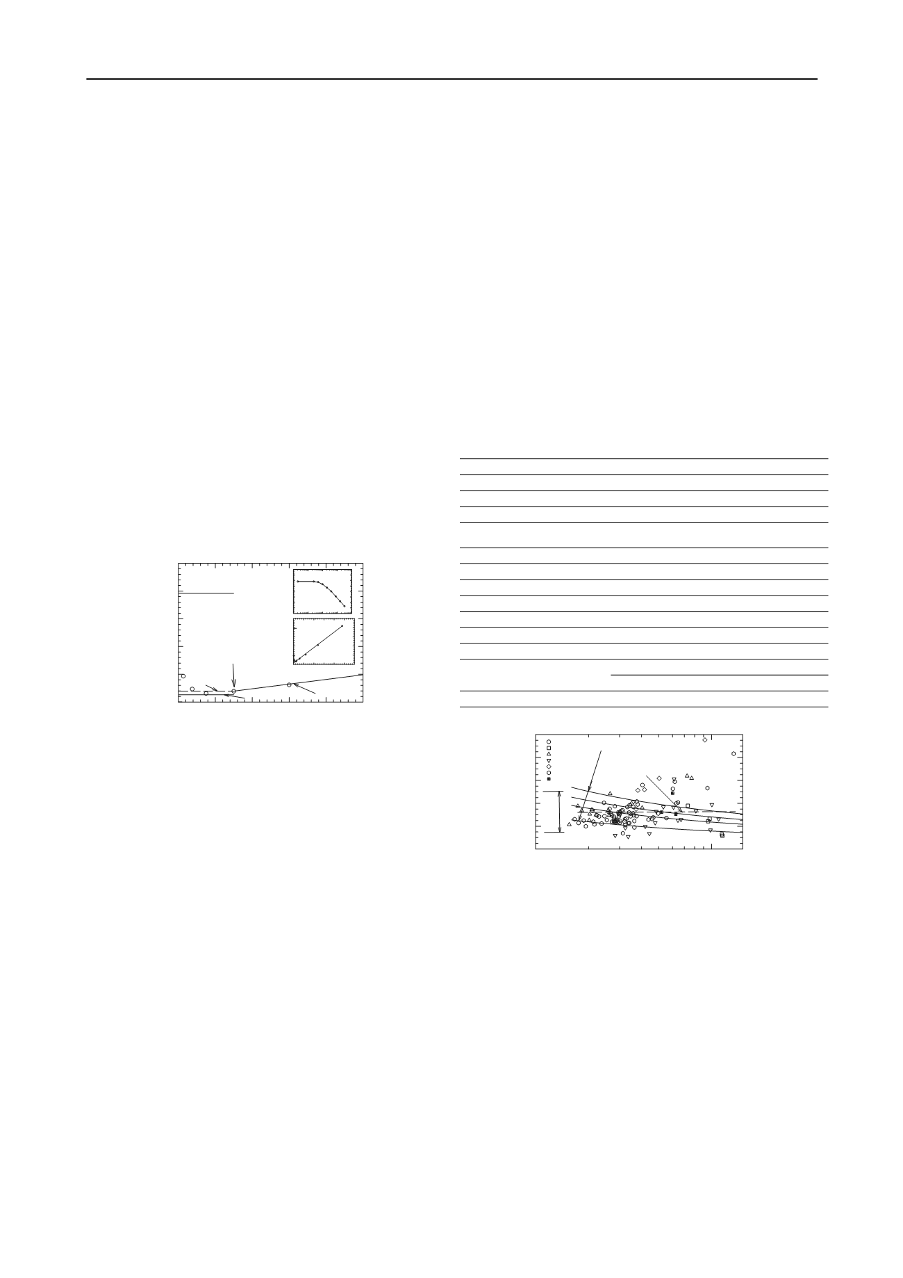
Friction Ratio, F
r
= [f
s
/(q
t
-
vo
)] 100, %
1
10
k =
'
p
/(q
t
-
vo
)
0.0
0.2
0.4
0.6
0.8
1.0
Idku
Metobus
Dammietta 3
Dammietta 4
PortSaid2
El-Gamil
Dammietta 2
Average k = 0.32
(q
t
-
5 6 7 8 9
4 3
2
vo
)/
'
vo
1
5
20
10
Robertson (2012)
Range From
Literature
4 PEIZOCONE PENETRATION TESTS
Piezocone Penetration Tests with pore water pressure
measurements (CPTU) were performed at the sites. A l0 cm
2
Piezocone was used to carry out the testing. Records were
made at 2 cm intervals. At each tested depth, cone resistance
(q
c
), pore water pressures behind cone (u
2
) and side friction (f
s
)
were measured. Typical CPTU records at some of the sites
under study are shown in Hight et al. (2000), Hamza et al.
(2003) and Hamza et al. (2005). The corrected tip resistance, q
t
,
can be calculated as q
t
=q
c
+(1-
)u
2
, where
is a cone
factor. The net cone resistance, q
n
, can be calculated as q
n
= q
t
-
vo
, where
vo
is the total overburden pressure.
5 PEIZOCONE PENETRATION TESTS
5.1. Stress History or Overconsolidation Ratio
Review of the available correlations between
’
p
or OCR and
Piezocone results was carried out by Lunne et al. (1997), Mayne
(2001), Ladd and DeGroot (2003), Powell and Lunne (2005),
Pant (2007), Mayne (2009), Becker (2010) and Robertson
(2012). The cone parameters used in the correlations include q
c
,
q
t
, q
t
-
vo
, q
t
-u
2
,
u. Some of these parameters were used with or
without normalization by
’
vo
. According to Campanella and
Robertson (1988), there is no unique relationship between OCR
or
’
p
and measured penetration induced pore water pressures
and if exists, it is poor because the pore pressures measured is
influenced by the location of the u measurement (i.e. u
1
, u
2
or
u
3
), clay sensitivity, over consolidation mechanism, soil type
and local heterogeneity. The most common and widely used
correlation is (e.g. Lunne et al. 1997):
’
p
= k (q
t
-
vo
) or OCR =
’
p
/
'
vo
= k(q
t
-
vo
)/
'
vo
(8)
It should be noted that empirical constant k in both
expressions in Equ. 8 is the same. Table (1) shows a summary
of k values reported in the literature. According to the table, k is
in the range of 0.14 to 0.5. Mayne (2001) showed that k is
slightly dependent on plasticity index, while Becker (2010)
showed that k is slightly dependent on coefficient of horizontal
pressure at rest. Robertson (2012) suggested an expression that
is dependent on (q
t
-
vo
)/
'
vo
and sleeve friction ratio, F
r
. The
empirical constant is calculated for the data in this study and is
plotted versus F
r
in Figure (5). The expression suggested by
Robertson (2012) was also plotted on the same plot. Figure (5)
shows that the Robertson (2012) predicts well the range of k.
However, it seems that k is slightly increasing with F
r
. The
calculated k values are in the range of 0.1 to 0.6 (0.18 to 0.4, if
scatter is ignored) with an average of 0.32, which is consistent
with the existing correlations in the literature.
Table 1. Summary of the parameter k from the literature..
Reference
k
Comment
Lefebvre & Poulin (1979)
0.25- 0.4
Norway & UK sites
Mayne & Holtz (1988)
0.4
World Data
Larson & Mulabdic (1991)
0.29
Scandinavian Soils
Mayne (1991)
0.33
Cavity Expansion & Critical
State Soil Mechanics Analysis
Leroueil et al. (1995)
0.28
Eastern Canada Clays
Chen & Mayne (1996)
0.305
205 Clay sites
Lunne et al. (1997)
0.2 – 0.5
Mayne (2001)
0.65(I
p
)
-0.23
Mesri (2004)
0.25 – 0.32
s
u
/
’
p
=constant interpretation
Abdelrahman et al. (2005)
0.2 – 0.5
Port Said Site, Egypt
Pant (2007)
0.14
Louisiana Soils – 7 Sites
Becker (2010)
0.3
Beaufort Sea Clays K
o
=1.5
0.24
Beaufort Sea Clays K
o
=2.0
Robertson (2012)
*
SHANSEP & CSSM
* k = [ [(q
t
-
vo
)/
’
vo
]
0.2
/ (0.25(10.5+7log F
r
)) ]
1.25
where F
r
= f
s
/(q
t
-
vo
)
Figure (5) Empirical constant k for the sites in this study
Ladd and De Groot (2003) proposed the following
SHANSEP type of expression to estimate OCR:
OCR = k
OCR
[(q
t
-
vo
)/
'
vo
]
1.25
(9)
Ladd and De Groot reported a value of 0.192 for k
OCR
based
Boston Blue clay experience. Robertson (2009) suggested
general k
OCR
value of 0.25. Robertson (2012) suggested the
expression in Equ. (10) to estimate k
OCR
based on F
r
:
k
OCR
= (2.625+1.75 log F
r
)
1.25
(10)
The data of Delta clay sites was used to back calculate k
OCR
and was plotted versus Fr in Fig. (6). The Robertson (2012)
expression was also plotted on Fig. (6). Figure (6) shows that
Equ. (10) predict well the range of k
OCR
. However, it seems that
k
OCR
is slightly increasing with F
r
. The average k
OCR
of the data
in this study was about 0.23 that is consistent with data in
literature.


