434
Proceedings of the 18
th
International Conference on Soil Mechanics and Geotechnical Engineering, Paris 2013
Soil Types
Symbol in
Figures Plastic
Limit (%)
Liquid
Limit (%)
Plasticity
Index
Particle
Density
(g/cm
3
)
Fujinomori
F
21.3
48.6
27.3
2.69
Kasaoka
K 27.5
62
33.5
2.61
NSF
N 29
55
26
2.76
Ariake
A 31.4
72.5
41.1
2.621
Hachirogata
H 96.5
246
149.5
2.43
Tokuyama
T
40
110.6
70.6
2.62
Table 1. Geotechnical Properties used in the test.
thin plastic film, and then it was kept in a high humidity box to
prevent the water evaporation. The elapsed time for thixotropy
was accounted just after the sample was poured into the mold.
As input signals for the bender element test, sine and
rectangular waves have been alternatively used with wide
ranges of frequencies in accordance with material stiffness, in
order to attain a clear output waveform. Generally, the high
frequency is required in testing stiff soils and vice versa. The
“start
-to-
start” method for de
termining the arrival time (
t
) and
“tip
-to-
tip” method for det
ermining the travel distances (
d
) of
the shear wave were adopted in this study (Yamashita et al.,
2009).
The increase in the undrained shear strength during
thixotropic hardening was also confirmed by the vane shear test.
The vane diameter and height used in this experiment were 20
mm and 40 mm, respectively. The shear rate of the laboratory
vane apparatus was constant at 6
rotations per minute. All tests
were carried out for the same sample created by a gallon bucket,
as already mentioned.
3 THIXOTROPIC EFFECT MEASUREMENT
3.1
Shear Wave Velocity and Shear Modulus by Bender
Element Test
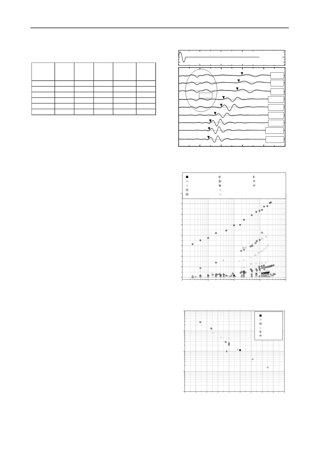
Figure 1 shows an example of increase in the shear wave
velocity (
V
s
) with time, measured by the bender element test on
a specimen made from Kasaoka clay mixed with 60.6% of
water content. Since the water content of the specimen was
almost equal to liquid limit state, the received shear wave
signals at the beginning of the measurement were hardly
identified because of their low amplitude and frequency. P-
waves clearly appeared since they could propagate through
liquid. As time was proceeded, the soil became stiffer;
consequently the arrival times were detected more shortly, in
another word the shear wave velocity increased. It may be
considered that the increase in shear wave velocity (
V
s
)
corresponds to the increases in the stiffness, which is reflected
to the thixotropic phenomenon. The received shear waves
became much clearer with high amplitude and frequency after a
certain time, while P-waves seemed to decay.
The shear modulus (
G
) derived from
V
s
with elapsed time is
illustrated in Fig. 2, where the symbols of A, F, K, N, H, and T
represent Ariake, Fujinomori, Kasaoka, NSF, Hachirogata, and
Tokuyama clays respectively with sample number. The number
in the brackets indicates the water content (
w
) and the
normalized water content by the liquid limit (
w
/
w
L
). It can be
seen from the figures that
G
values for all conditions increases
with time even at over limit liquid states. And,
G
builds up
nearly in proportion to time in the logarithm scale, but this
magnitude is certainly depended on types of soils and the
amount of water content.
Since
G
increases in time,
G
at 24 hrs (
G
24
) will be a
represented parameter for identifying characteristics of soil
types and influence of water content.
G
24
is plotted in Fig. 3
Figure 1. An example of shear waves (Kasaoka clay,
w
=60.6%)
Figure 2. Relationships between G and time.
Figure 3. Relationship between
w
/
w
L
and
G
after 24 hours.
against the (
w
/
w
L
), considering different types of materials. A
clear correlation between these two parameters can be observed
0
3
6
9
12
15
-10
0
10
P-waves
142.0 hrs
116.8 hrs
93.8 hrs
44.4 hrs
23.7 hrs
19.5 hrs
2.7 hrs
2.2 hrs
Time (ms)
1.5 hrs
Voltage (V)
Input Signal
Sine 1 kHz
0.1
1
10
100
1000
0
500
1000
1500
2000
2500
3000
3500
4000
A1 (79.8%; 1.10)
K3 (52.0%; 0.84)
H1 (241.3%; 0.98)
F1 (40.9%; 0.84)
K4 (62.1%; 1.00)
T1 (134.3%; 1.21)
F2 (52.5%; 1.08)
K5 (46.0%; 0.74)
T2 (149.3%; 1.35)
K1 (62.3%; 1.00)
N1 (54.0%; 0.93)
K2 (60.6%; 0.97)
N2 (48.6%; 0.86)
Shear Modulus,
G
(kPa)
Time (hr)
0.6 0.7 0.8 0.9 1.0 1.1 1.2 1.3 1.4 1.5
1
10
100
1000
10000
Ariake
Fujinomori
Kasaoka
NSF
Hachirogata
Tokuyama
Shear Modulus at 24hrs,
G
24
(kPa)
Normalized
w
/
w
L


