405
Technical Committee 101 - Session II /
Comité technique 101 - Session II
a
of about 12%, but thereafter, vertical symmetry was
broken. Associated with this deformation,
q
deviated from the
perfect path and exhibited small values.
(a) 5% 10% 15% 20%
(b) 5% 10% 15% 20%
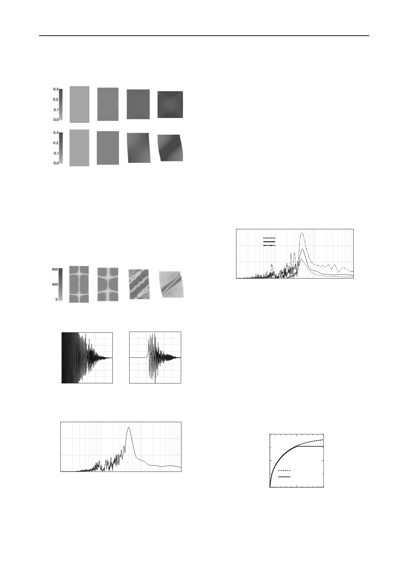
Fig. 5 Change in shear strain distribution in a specimen with initial
imperfection in top loading
(a) No initial imperfections. (b) With initial imperfections.
4.2
ACCELERATIONS ASSOCIATED WITH SHEAR
BANDING AND THEIR FOURIER AMPLITUDES
Fig. 6 shows the distribution of the horizontal component of
acceleration generated in the specimen in (b). The acceleration
distribution is symmetrical left to right and top to bottom up to
about an
a
of 12%. These are the accelerations generated due
to the compression from the top and bottom as described above.
In contrast, after the breakdown of vertical symmetry, localized
5% 10% 15% 20%
Fig. 6 Occurrence of shear banding associated with horizontal
components of generated accelerations (gal)
0
0.08
0.16
0.24
–2000
–1000
0
1000
2000
Time(sec)
Acceleration(gal)
0
0.08
0.16
0.24
–2000
–1000
0
1000
2000
Time(sec)
Acceleration(gal)
(i) Horizontal component
(ii) Vertical component
Fig. 7 (i) Horizontal component and (ii) vertical component of
acceleration generated at the side surface of the specimen
0.0001
0.001
0.01
0.1
0
4
8
12
Fourier amplitude [gal*s]
Period T [sec]
Fig. 8 Fourier amplitude of the vertical component of accelerations
generated at point A
shear banding developed like reverse faults, and accelerations
were generated along the shear bands. Fig. 7 shows (i) the
horizontal component and (ii) the vertical component of
acceleration generated at the node A shown in Fig. 1. Different
from the horizontal component of acceleration, the vertical
component was the component normal to the central axis of the
specimen, and kept to be zero until about 0.08 sec after the start
of loading, in other words, until the
a
was about 10%.
Thereafter, as the shear banding started, new accelerations were
generated with a maximum value of about 2000 gal. Also, after
exhibiting the maximum value of acceleration, each component
tended to converge as
a
increased. Fig. 8 shows the Fourier
amplitude of the acceleration up to
a
= 30% for the side
surface (point A) of the specimen. From these figures, it can be
seen that accelerations are generated predominantly with a
period of around 5.0×10
-3
sec.
5 LOADING RATE EFFECT
An investigation into the effect of displacement rate was carried
out for compression under displacement control by applying a
geometric initial imperfection in (b) of section 4. Fig. 9 shows
the results of a comparison of the Fourier amplitudes of the
accelerations obtained at point A on the side surface of the
specimen for displacement velocities of 2.5 cm/s, 5 cm/s, and
10 cm/s. In all cases, the specimen deformed as in Fig. 5(b)
(figures omitted). From Fig. 9, it can be seen that the Fourier
amplitudes increase with velocity, as a loading rate effect, and
that the predominant vibration amplitude is about 5.0×10
-3
sec
with almost no variation.
0.0001
0.001
0.01
0.1
0
6
12
18
Fourier amplitude [gal*s]
Period T [sec]
2.5 cm/s
5.0 cm/s
10.0 cm/s
Fig. 9 Fourier amplitude of the vertical component of acceleration
generated at point A on the right side surface of the specimen (load rate
effect)
6 UNDRAINED CREEP BEHAVIOR UNDER CONSTANT
LOAD
In this section, firstly all the initial and boundary conditions as
well as the initial imperfection are same as (b) in section 4. The
calculation performed was continued after deviation from the
perfect path until (i)
a
=13% (0.104 sec after the start) and (ii)
a
=18.75% (0.150 sec after the start), and then was altered to
load control at the top, maintaining the load constant, and
continuing with displacement control on the bottom edge but
stopping the vertical displacement. For load control, the
conditions for the pedestal with no friction were calculated
using the
constraint conditions on the finite element nodes by
the Lagrange method of undetermined multipliers, as in Asaoka
et al. 1998. The results of the calculations are described below.
0
0.1
0.2
500
1000
Time (sec)
Deviator stress
q
(kPa)
Perfect path
Imperfection path
Fig. 10 Load control after displacement control (“creep”)
Fig. 10 shows the relationship between the calculated
specimen apparent top
q
and the elapsed time from
displacement control, and Fig. 11 shows the change in axial
strain from the start of displacement control. However, in Fig.
10,
q
was obtained by dividing by the initial area of the top of
the specimen. Also, the ○ in Fig. 11 indicates the point of


