404
Proceedings of the 18
th
International Conference on Soil Mechanics and Geotechnical Engineering, Paris 2013
overconsolidation degradation index
m
, which controls the
overconsolidation behavior, the elasto-plastic constants used
were the same values as used by Asaoka et al. 1994. Vertical
constant loading rate was applied on the top surface. The
boundary conditions were assumed to be constant lateral
pressure and undrained conditions, with no friction at the top
and bottom and with complete freedom of movement in the
horizontal direction. Calculation under these conditions cannot
be realized with quasi-static analysis that ignores inertial forces.
The mesh subdivision was 70 elements laterally by 160
elements vertically.
Table 1 Specimen elasto-plastic constants and initial values
Elasto-plastic parameters
Critical state index M
1.55
NCL intercept N
2.0
Compression index
λ,˜
0.108
Swelling index
κ,˜
0.025
Poisson's ratio ν
0.3
Evolution parameters
Degradation index of OC
m
0.2
Initial conditions
Specific volume v
0
1.747
Stress ratio
η
0
0.0
Degree of structure 1
/R
0
�
1.0
Degree of overconsolidation 1
/R
0
5.0
Degree of anisotropy ζ
0
0.0
Soil particle density
ρ
s
(g/cm
3
)
2.65
Permeability coefficient
k
(cm/s)
3.7×10
-8
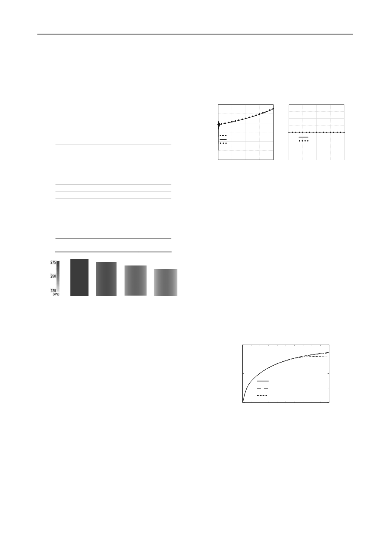
5% 10% 15% 20%
Fig. 2 Change in specimen deformation and pore water pressure
distribution under uniform deformation
3 REPRODUCTION OF A UNIFORM FIELD USING THE
GEOASIA ANALYSIS CODE
Consider undrained compression deformation of a perfectly
rectangular specimen with no initial material or geometric
imperfections. The top and bottom of the specimen were free in
the horizontal direction, and after fixing the bottom in the
vertical direction, a constant uniform vertical displacement was
applied to the top. In accordance with the
u
-
p
Formulation,
when solving without ignoring inertial forces, a uniform
deformation field satisfying element-wise undrained conditions
in a rectangular specimen can only be realized when the
permeability coefficient is
, although the theoretical proof
(Noda et al. 2013) is omitted. In order to realize a uniform
deformation field using this analysis code, it is necessary to set
a velocity distribution that is proportional to the height and the
velocity applied to the top of the specimen (not all are zero), an
acceleration distribution to maintain the rectangular shape, and
pore water pressures that exhibit a parabolic distribution in the
horizontal direction as initial conditions in addition to the
coordinates of the finite element nodes at the boundary and
interior (Noda et al. 2013).
0
k
In this section, for the case with
first, a constant
vertical velocity of 10
3
cm/s was applied on the top to illustrate
the calculation results when a uniform deformation field is
achieved. Fig. 2 shows the change in specimen deformation and
the parabolic pore water pressure distribution, and Fig. 3 shows
the horizontal component and vertical component of
acceleration generated in the center of the right side surface of
the specimen. However, when the theoretical initial values are
set for the velocity and acceleration as initial conditions, small
vibrations occur around time
t
=0. Therefore, for no vibration the
initial velocities and accelerations are set slightly smaller than
the theoretical values. See Noda et al. 2013 for the method of
obtaining the reduced values.
0
k
0
0.0008
0.0016
–60000
0
60000
120000
Time(sec)
Acceleration(gal)
Computed (Reduced values)
Theoretical result
(1.6E+05)
Computed (Non–reduced values)
0
0.0008
0.0016
–1
–0.5
0
0.5
1
Time(sec)
Acceleration(gal)
Computed result
Theoretical result
(1.6E+05)
(i) horizontal (ii) vertical
Fig. 3 Difference in acceleration generated at the right side surface of
the specimen
4 OCCURRENCE OF ACCELERATION ASSOCIATED
WITH SHEAR BANDING
In the following, the initial conditions were changed from the
conditions appropriate to realize a uniform deformation field to
velocities, accelerations, and pore water pressures that are all
zero. The calculation was carried out with (a) no initial
geometric imperfections and (b) initial geometric imperfections
applied to the specimen. In the case of (b), a half wavelength
cosine curve (primary mode) with a small amplitude of 10
-5
cm
was applied to the side surfaces of the specimen in accordance
with Asaoka et al. 1994. In static analysis, as in Asaoka et al.
1994, this is the shape of the induced initial imperfection, and it
changed to the primary mode with reduction in load
(imperfection-sensitive bifurcation behavior). In this section, in
order for the specimen to maintain vertical symmetry in the case
of (a), a vertical displacement at the constant rate of 0.5×10
cm/s was applied to both the top and bottom of the specimen in
the compression direction. Also, the permeability coefficient
was changed from zero to the values shown in Table 1. The
calculation results are shown below.
0
10
20
500
1000
Axial strain
a
(%)
Deviator stress
q
(kPa)
Perfect path
Imperfection path, (b)
Non–imperfection path, (a)
Fig. 4 Relationship between apparent
q
-
with differences in initial
imperfections
a
4.1
VERTICALLY ASYMMETRIC DEFORMATION
INDUCED BY INITIAL IMPERFECTIONS
Fig. 4 shows the apparent axial differential stress
q
– axial strain
a
relationship, and Fig. 5 shows the specimen shear strain
distribution.
q
is the total increment of equivalent nodal forces
obtained on the top divided by the area of the top at each time,
and
a
is the vertical displacement divided by the initial
height. In the case of (a),
q
was virtually the same as the
“perfect path” (= response of the constitutive equation) obtained
in the uniform deformation field, and the specimen maintained
left to right and top to bottom symmetry from the beginning to
end. In contrast, in the case of (b), the deformation virtually
maintained left to right and top to bottom symmetry up to an


