38
Proceedings of the 18
th
International Conference on Soil Mechanics and Geotechnical Engineering, Paris 2013
Proceedings of the 18
th
International Conference on Soil Mechanics and Geotechnical Engineering, Paris 2013
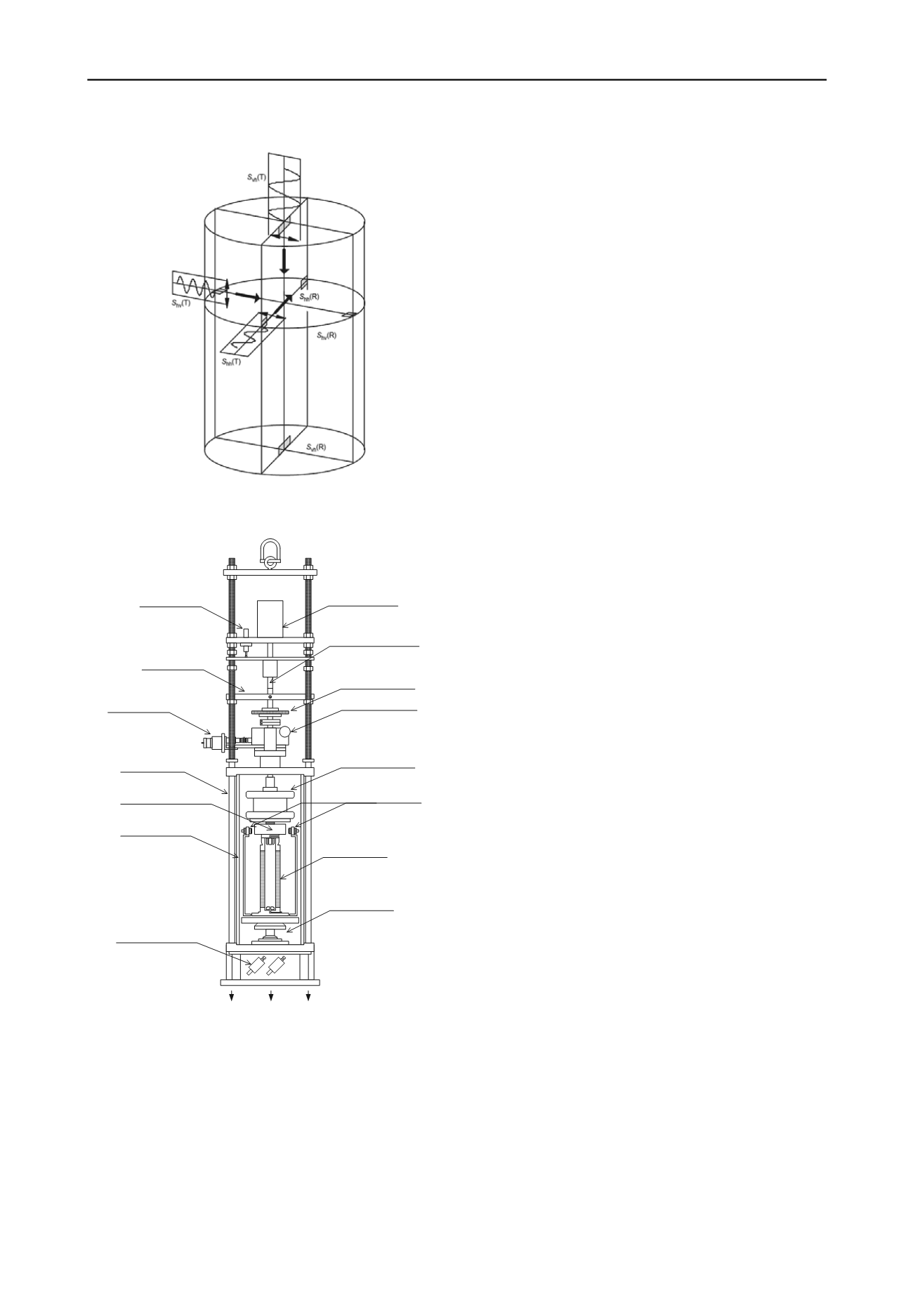
Fig. 6. Bender element configuration to investigate stiffness of sands:
Kuwano and Jardine 1998, 2002a
Bellofram cylinder
Hardin oscillator
Specimen
Load cell
Proximity transducers
Tie rod
Acrylic chamber wall
Stepper motor for
torsion
Cam
Outer cell and pore water
pressure transducers
Sprocket and torque
transmission chain
Displacement
Transducer
Clamp
To foundation
Rotary tension cylinder
Ram
Fig. 7. Schematic arrangements of Resonant-Column HCA system
employed to test sands: Nishimura et al 2007
Kuwano and Jardine 1998, 2002a,b noted the high sensor
resolution and stability required to track sands’ stress-strain
responses from their (very limited) pseudo-elastic ranges through
to ultimate (large strain) failure. Even when the standard
deviations in strain measurements fall below 10
-6
, and those for
stresses below 0.05kPa, multiple readings and averaging are
required to establish initial stiffness trends. Highly flexible
stress-path control systems are also essential.
Kuwano and Jardine 2007 emphasise that behaviour can only
be considered elastic within a very limited kinematic hardening
(Y
1
) true yield surface that is dragged with the current effective
stress point, growing and shrinking with p΄ and changing in
shape with proximity to the outer, Y
3
surface; Jardine 1992. The
latter corresponds to the yield surface recognised in classical
critical state soil mechanics. Behaviour within the true Y
1
yield
surface is highly anisotropic, following patterns that evolve if K,
the ratio of the radial to vertical effective stress (K = σ΄
r
/σ΄
z
),
changes. Plastic straining commences once the Y
1
surface is
engaged and becomes progressively more important as straining
continues along any monotonic path. An intermediate kinematic
Y
2
surface was identified that marks: (i) potential changes in
strain increment directions, (ii) the onset of marked strain-rate or
time dependency and (iii) a threshold condition in cyclic tests (as
noted by Vucetic 1994) beyond which permanent strains (or p΄
reductions in constant volume tests) accumulate significantly.
The Y
3
surface is generally anisotropic. For example, the
marked undrained shear strength anisotropy of sands has been
identified in earlier HCA studies (Menkiti 1995, Porovic 1995,
Shibuya et al 2003a,b) on HRS. The surface can be difficult to
define under drained conditions where volumetric strains
dominate. Kuwano and Jardine 2007 suggested that its evolution
could be mapped by tracking the incremental ratios of plastic to
total strains. They also suggested that the Phase Transformation
process (identified by Ishihara et al 1975, in which specimens
that are already yielding under shear in a contractant style could
switch abruptly to follow a dilatant pattern) could be considered
as a further (Y
4
) stage of progressive yielding. Jardine et al
2001b argue that the above in-elastic features can be explained
by micro-mechanical grain contact yielding/slipping and force
chain buckling processes. The breakage of grains, which
becomes important under high pressures, has also been referred
to as yielding: see Muir-Wood 2008 or Bandini and Coop 2011.
HCA testing is necessary to investigate stiffness anisotropy
post-Y
1
yielding; Zdravkovic and Jardine 1997. However, cross-
anisotropic elastic parameter sets can be obtained within Y
1
by
assuming rate independence and combining very small-strain
axial and radial stress probing experiments with multi-axis shear
wave measurements. Kuwano 1999 undertook hundreds of such
tests under a wide range of stress conditions, confirming the
elastic stiffness Equations 1 to 5. Ageing periods were imposed
in all tests before making any change in stress path direction to
ensure that residual creep rates reduced to low proportions
(typically <1/100) of those that would be developed in the next
test stage. Note that the function used to normalise for variations
in void ratio (e) is f (e) = (2.17 – e)
2
/(1 + e).
u
B
r
u
u
ppAef
E
/ .
). (
(1)
v
C
r
v v
v
p
Aef
E
/
. ). (
'
'
(2)
h
D
r
h h
h
p
Aef
E
/
.
). (
'
'
(3)
vh
vh
D
r
h
C
r
v
vh
vh
p
p
Aef
G
/
.
/
.
). (
'
'
(4)
hh
hh
D
r
h
C
r
v
hh
hh
p
p
Aef
G
/
.
/
.
). (
'
'
(5)
The terms A
ij
, B
ij
, C
ij
and D
ij
are non-dimensional material
constants and p
r
is atmospheric pressure. With Dunkerque sand
the values of B
u
and the sum [C
ij
+ D
ij
] of the exponents
applying to Equations 1 to 5 fell between 0.5 and 0.6. The
equations are evaluated and plotted against depth in Fig. 8
adopting Kuwano’s sets of coefficients (A
ij
, B
ij
, C
ij
and D
ij
)
combined with the Dunkerque unit weight profile, water table
depth and an estimated K
0
= 1 – sin φ΄ for the normally
consolidated sand. A single void ratio (0.61) has been adopted
for this illustration that matches the expected mean, although the
CPT q
c
profiles point to significant fluctuations with depth in
void ratio and state. Also shown is the in-situ G
vh
profile
measured with seismic CPT tests and DMT tests conducted by
the UK Building Research Establishment (Chow 1997).


