3357
Technical Committee 307 + 212 /
Comité technique 307 + 212
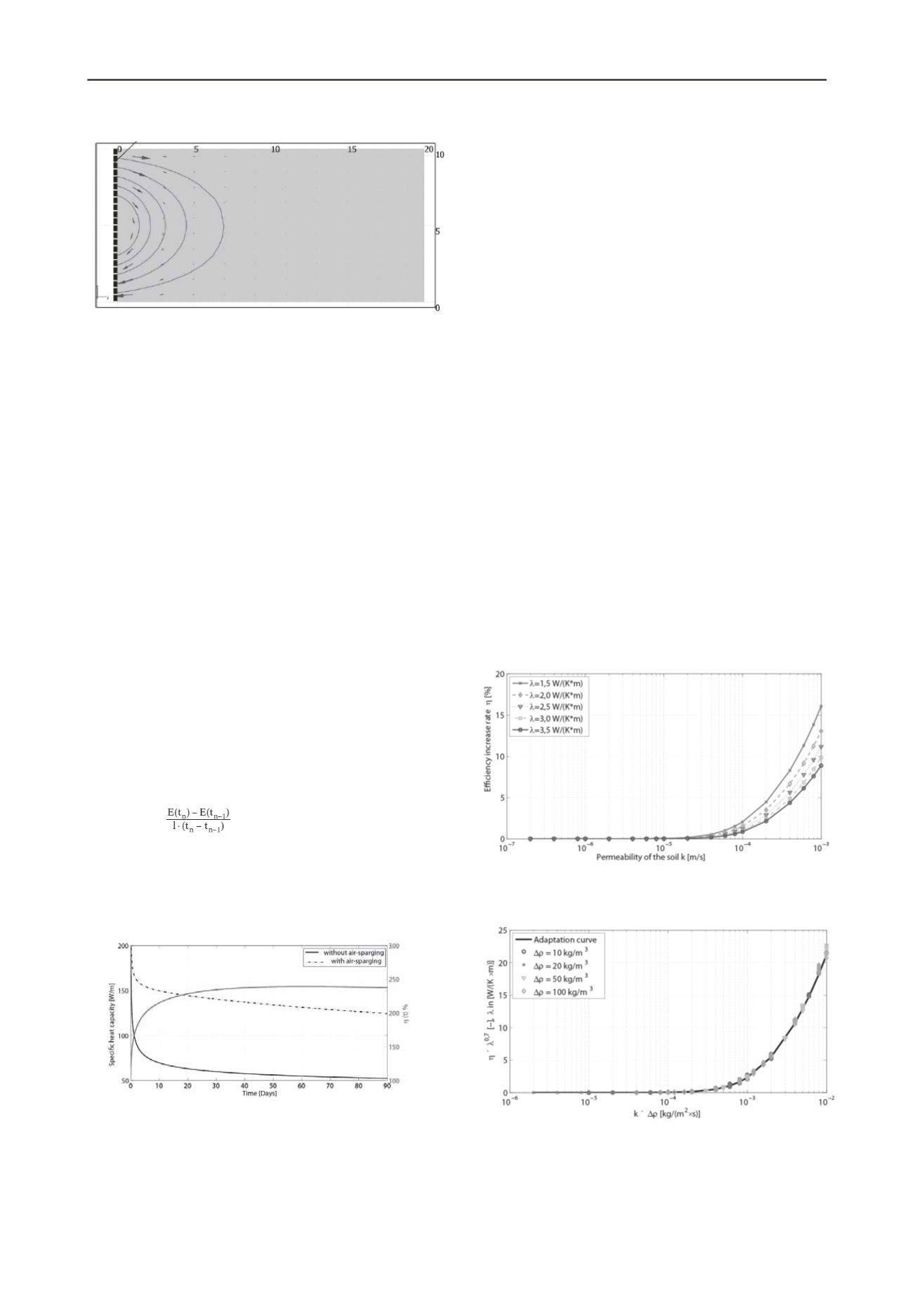
Figure 4. calculated velocity field (arrows) and particle tracing (lines) of
the groundwater around the air-sparging downhole heat exchanger at a
steady rate (Δρ = 10 kg/m³, k = 10
-4
m/s)
3.2
Heat transport
Without the air injection the heat distribution around the
borehole heat exchanger is uniform. The induced groundwater
circulation transports heat away from the well and changes the
shape of the temperature field. In the upper part of the aquifer
the convective heat transport has the same direction as the
conductive heat transport. This increases the heat spreading rate,
which can be seen from the larger heat plume around the well.
In the lower part of the well the groundwater flow direction is
opposite the direction of heat conduction, which slows the heat
spreading rate. At the bottom of the well the groundwater flow
towards the well is so strong that the heat cannot spread
outwards anymore.
The overall heat plume around the well is larger when air
injection is active. This shows that more heat can be transported
into the ground using an air-injection borehole heat exchanger
than using a regular borehole heat exchanger.
3.3
Efficiency of air-injection borehole heat exchanger with
standard parameters
The amount of heat E(t
n
) that the borehole heat exchanger
transports into the ground at the time t
n
equals the integral
product of the temperature change along the entire body of soil
with a soil density of ρ
B
and the specific heat capacity c
B
:
E(t
n
) = ∫ρ
B
c
B
[T(x,y,z,t
n
) – T
0
]dV
(1)
The specific heat abstraction capacity per meter heat exchanger
P
s
(t
n
) is time-dependent:
P
S
(T
N
) =
(2)
In this case l is the length of the borehole heat exchanger.
Figure 5 shows the specific heat abstraction capacity as a
function of time, comparing a regular borehole heat exchanger
and one that uses air injection. In both systems the heat
abstraction capacity rapidly reduces within 20 days and changes
only minimally afterwards.
Figure 5. Calculated specific heat capacity with and without air sparging
and efficiency increasing rate of the downhole heat exchanger compared
with normal downhole heat exchanger (Δρ = 10 kg/m³, λ = 2.5 W/(m ·
K), k = 10
-4
m/s)
3.4
Variation calculations
During the calculations three parameters were varied: density of
the air-water-mixture inside the well, heat conductivity and
permeability of the soil.
For low permeabilities of the soil (k < 10
-5
m/s) the heat
abstraction capacity depends only on the thermal conductivity
of the soil. In permeable soils (k > 10
-4
m/s), convection is the
dominant heat transport mechanism and heat conduction has no
influence. In between those parameters the heat abstraction
capacity depends on permeabilty as well as on thermal
conductivity.
The influence of the air injection depends on the ratio
between thermal conductivity and induced convection. The
decisive factor for thermal conductivity is the specific thermal
conductivity of the soil (λ). The convection depends on the
median groundwater circulation velocity (v
z
) that can be
calculated using Darcy’s law.
v
z
= k · i
(3)
Assuming a constant median flow distance the following
relationship can be applied:
v
z
= c · k · Δρ
(4)
Here, c is a constant. The efficiency increasing rate (η) is
therefore mainly dependent on the three parameters k, λ and Δρ.
The relationship between η and λ shows that the five curves in
Figure 6 fit very well when η is mutlilied by λ
0.7
. The
relationship between η, λ, k and Δρ is shown in Figure 7. The y-
axis is labeled η · λ
0.7
and the x-axis is labeled k · Δρ. All
calculated points can be converged towards the adaptation
curve.
Figure 6. Calculated efficiency increasing rate of the air-sparging
downhole heat exchanger against the conductivity and permeability of
the soil (Δρ = 10 kg/m³)
Figure 7. Presentation of the results of the variation calculations and the
adaptation curve, x-axis: k · Δρ, y-axis: η · λ
0.7
This phenomenon offers the possibility of estimating the
efficiency increasing rate when the three parameters λ, k and Δρ
are known.
Figure 5. Calculated specific heat capacity with and without air sparging
and efficiency increasing rate of the downhole heat exchanger compared
with normal downhole heat exchanger (Δρ = 10 kg/m³, λ = 2.5 W/(m ·
K), k = 10
-4
m/s)
3.4
Vari tion calculations
Figure 7.
adaptatio
This ph
efficienc
are kno
Figure 4. calculated velocity field (arrows) and particle tracing (lines) of
the groundwater around the air-sparging downhole heat exchanger at a
steady rate (Δρ = 10 kg/m³, k = 10
-4
m/s)
3.2
Heat transport
Without the air injection the heat distribution around the
borehole heat exchanger is uniform. The induced groundwater
circulation transports heat away from the well and changes the
shape of the temperature field. In the upper part of the aquifer
the convective heat transport has the same direction as the
conductive heat transport. This increases the heat spreading rate,
which can be seen from the larger heat plume around the well.
In the lower part of the well the groundwater flow direction is
opposite the direction of heat conduction, which slows the heat
spreading rate. At the bottom of the well the groundwater flow
towards the well is so strong that the heat cannot spread
outwards anymore.
The overall heat plume around the well is larger when air
injection is active. This shows that more heat can be transported
into the ground using an air-injection borehole heat exchanger
than using a regular borehole heat exchanger.
3.3
Efficiency of air-injection borehole heat exchanger with
standard parameters
The amount of heat E(t
n
) that the borehole heat exchanger
transports into the ground at the time t
n
equals the integral
product of the temperature change along the entire body of soil
with a soil density of ρ
B
and the specific heat capacity c
B
:
E(t
n
) = ∫ρ
B
c
B
[T(x,y,z,t
n
) – T
0
]dV
(1)
The specific heat abstraction capacity per meter heat exchanger
P
s
(t
n
) is time-dependent:
P
S
(T
N
) =
(2)
In this case l is the length of the borehole heat exchanger.
Figure 5 shows the specific heat abstraction capacity as a
function of time, comparing a regular borehole heat exchanger
and one that uses air injection. In both systems the heat
abstraction capacity rapidly reduces within 20 days and changes
only minimally afterwards.
Figure 5. Calculated specific heat capacity with and without air sparging
and efficiency increasing rate of the downhole heat exchanger compared
with normal downhole heat exchanger (Δρ = 10 kg/m³, λ = 2.5 W/(m ·
K), k = 10
-4
m/s)
3.4
Variation calculations
During the calculations three parameters were varied: density of
the air-water-mixture inside the well, heat conductivity and
permeability of the soil.
For low permeabilities of the soil (k < 10
-5
m/s) the heat
abstraction capacity depends only on the thermal conductivity
of the soil. In permeable soils (k > 10
-4
m/s), convection is the
dominant heat transport mechanism and heat conduction has no
influence. In between those parameters the heat abstraction
capacity depends on permeabilty as well as on thermal
conductivity.
The influence of the air injection depends on the ratio
between thermal conductivity and induced convection. The
decisive factor for thermal conductivity is the specific thermal
conductivity of the soil (λ). The convection depends on the
median groundwater circulation velocity (v
z
) that can be
calculated using Darcy’s law.
v
z
= k · i
(3)
Assuming a constant median flow distance the following
relationship can be applied:
v
z
= c · k · Δρ
(4)
Here, c is a constant. The efficiency increasing rate (η) is
therefore mainly dependent on the three parameters k, λ and Δρ.
The relationship between η and λ shows that the five curves in
Figure 6 fit very well when η is mutlilied by λ
0.7
. The
relationship between η, λ, k and Δρ is sho n in Figure 7. The y-
axis is labeled η · λ
0.7
and the x-axis is labeled k · Δρ. All
calculated points can be converged towards the adaptation
curve.
Figure 6. Calculated efficiency increasing rate of the air-sparging
downhole heat exchanger against the conductivity and permeability of
the soil (Δρ = 10 kg/m³)
Figure 7. Presentation of the results of the variation calculations and the
adaptation curve, x-axis: k · Δρ, y-axis: η · λ
0.7
This phenomenon offers the possibility of estimating the
efficiency increasing rate when the three parameters λ, k and Δρ
are known.


