2578
Proceedings of the 18
th
International Conference on Soil Mechanics and Geotechnical Engineering, Paris 2013
-1
n 1
1
X'C X
2 2
2
f (X) C (2 ) e
(1)
where C is the correlation matrix. For n = 3, the correlation
matrix is given by:
12
13
12
23
13
23
1
C
1
1
(2)
between X
i
and X
j
(not equal to the correlation between the
original physical variable Y
i
and Y
j
). It is clear that the full
multivariate dependency structure of a normal random vector
only depends on a correlation matrix (C) containing bivariate
correlations between all possible pairs of components, namely
X
1
and X
2
, X
1
and X
3
, and X
2
and X
3
. It is not necessary to
measure X
1
, X
2
, and X
3
simultaneously
. The practical advantage
of capturing multivariate dependencies in any dimension (i.e.,
any number of random variables) using only bivariate
dependency information is obvious.
It is simple to obtain realizations of
independent
standard
normal random variables U = (U
1
, U
2
, U
3
)
using library
functions in many softwares. Realizations of
correlated
standard normal random variables X = (X
1
, X
2
, X
3
)
can be
obtained using X = LU, in which L is the lower triangular
Cholesky factor satisfying C = LL
. Finally, each soil parameter
is obtained using Y
i
= F
-1
[
(X
i
)].
2.1
Complete multivariate information (structured clays)
A multivariate database of Y
1
= LI (liquidity index), Y
2
= s
u
, Y
3
= s
u
re
(remolded undrained shear strength), Y
4
=
’
p
(preconsolidation stress), and Y
5
=
’
v
(effective vertical stress)
is complied in Ching & Phoon (2012a). There are 345 data
points of structured clays from 37 sites worldwide, covering a
wide range of sensitivity, LI, and clay types, with simultaneous
knowledge of (Y
1
,Y
2
, …Y
5
)
. The OCR values of the data
points are generally small, mostly less than 4. Fissured and
organic clays are mostly left out of the database. Because s
u
values depend on stress state, strain rate, sampling disturbance,
etc., all s
u
values are converted into mobilized s
u
values
following the recommendations made by Mesri and Huvaj
(1997). The marginal probability density functions (PDF) for
(Y
1
,Y
2
, …Y
5
)
and their statistics (mean of Y
i
=
i
, COV of Y
i
=
V
i
, mean of ln(Y
i
) =
i
, standard deviation of ln(Y
i
) =
i
) are
summarized in Table 1.
For lognormal Y, the CDF transform is:
i
i
i
X ln Y
i
(3)
The transformed (X
1
, X
2
, …, X
5
)
are individually standard
normal random variables. The correlation matrix C for (X
1
, X
2
,
…X
5
)
is shown in Table 2, and (X
1
, X
2
, …X
5
)
is assumed to be
multivariate normal with the correlation matrix listed in the
table.
The multivariate normal distribution is employed to
simulate samples of (LI, s
u
, s
u
re
,
’
p
,
’
v
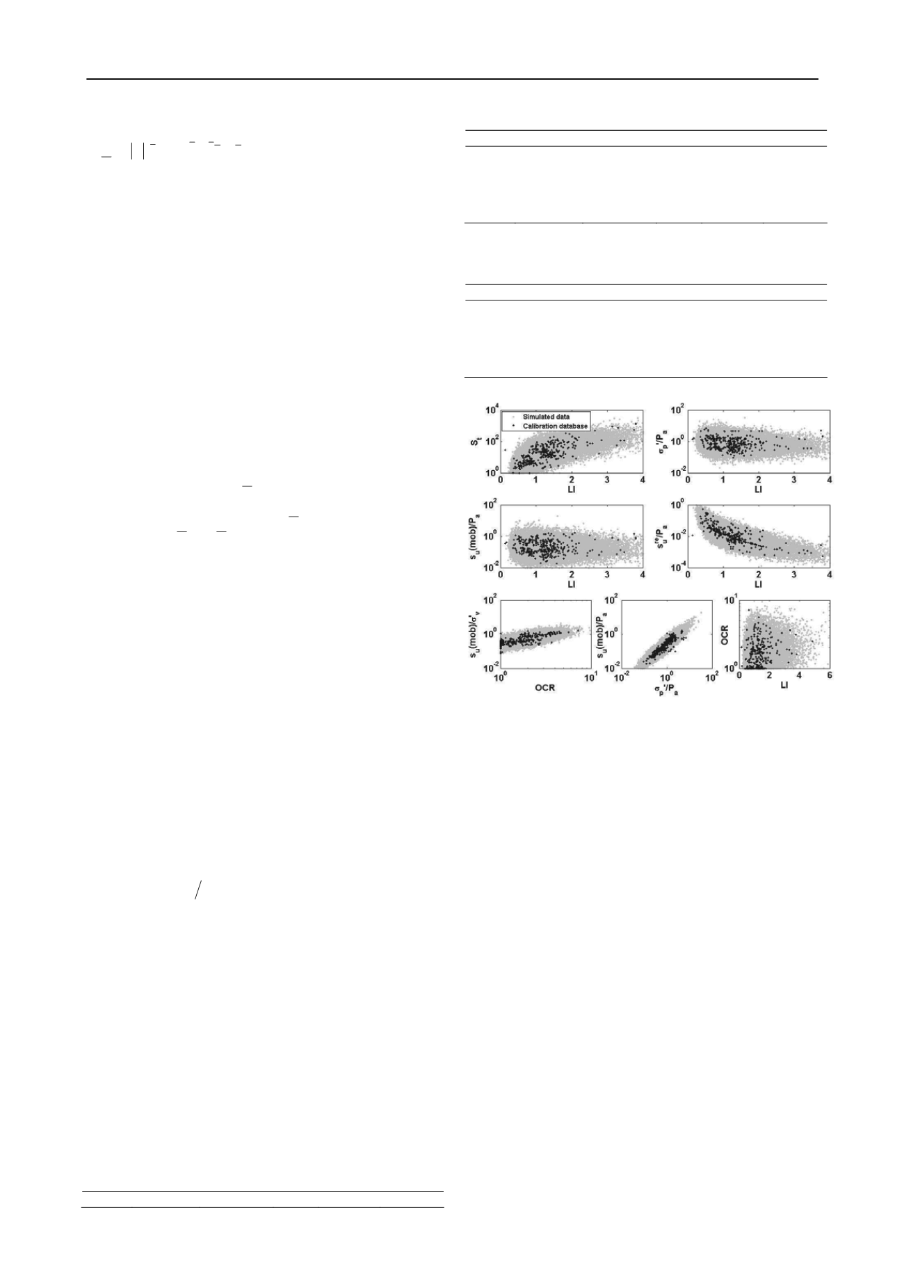
), shown in Figure 1
together with the calibration database. Not only the correlations
among the original random variables (LI, s
u
, s
u
re
,
’
p
,
’
v
) are
shown but the correlations among their derived (normalized)
quantities, including S
t
= s
u
/s
u
re
, OCR =
’
p
/
’
v
, s
u
/
’
v
, are also
shown. The multivariate normal distribution performs
adequately, as the simulated samples closely mimic the
correlation behaviors of the calibration database, even for those
with nonlinear trends, e.g. LI-s
u
re
and LI-S
t
correlations.
Table 1. Distributions and statistics of (Y
1
, Y
2
, …Y
5
)
for
structured clays (Source: Ching & Phoon 2012a).
Distribution
Mean
COV
Mean of
stdev of
ln(Y
i
),
i
ln(Y
i
),
i
Y
1
= LI Lognormal 1.25
0.49
0.122
0.459
Y
2
= s
u
Lognormal 31.01kN/m
2
0.95
3.051
0.898
Y
3
= s
u
re
Lognormal 2.51kN/m
2
1.52
0.226
1.191
Y
4
=
’
p
Lognormal 105.82kN/m
2
0.98
4.311
0.835
Y
5
=
’
v
Lognormal 66.63kN/m
2
0.80
3.891
0.823
Table 2. Correlation matrix C for (X
1
, X
2
, … X
5
)
for the five
selected parameters of structured clays (Source: Ching & Phoon
2012a).
X
1
(LI) X
2
(s
u
)
X
3
(s
u
re
)
X
4
(
’
p
)
X
5
(
’
v
)
X
1
(LI)
1.000
-0.083
-0.824
-0.176
0.280
X
2
(s
u
)
-0.083
1.000
0.276
0.915
0.801
X
3
(s
u
re
)
-0.824
0.276
1.000
0.365
0.453
X
4
(
’
p
)
-0.176
0.915
0.365
1.000
0.850
X
5
(
’
v
)
0.280
0.801
0.453
0.850
1.000
Figure 1. Comparisons between the calibration database and the
simulated data points (Source: Ching & Phoon 2012a).
2.2
Incomplete multivariate information (unstructured clays)
Ching et al. (2010) presented another clay database containing
four soil parameters: Y
1
= OCR, Y
2
= s
u
from CIUC test, Y
3
=
q
T
-
v
(net cone resistance), and Y
4
= N
60
(SPT N corrected for
energy efficiency). The range of OCR of this database is
wider – from 1 to 50. However, only bivariate data on (Y
1
, Y
2
)
= (OCR, s
u
), (Y
3
, Y
2
) = (q
T
-
v
, s
u
), and (Y
4
, Y
2
) = (N
60
, s
u
) are
available. Bivariate data on (Y
1
, Y
3
) = (OCR, q
T
-
v
), (Y
1
, Y
4
)
= (OCR, N
60
), and (Y
3
, Y
4
) = (q
T
-
v
, N
60
) are missing, i.e., the
bivariate correlations
ij
are only partially known. Given that
complete bivariate information is not available, it is not possible
to apply the aforementioned CDF transform approach directly.
It is accurate to say that although it is common to measure more
than two soil parameters in a site investigation, it is uncommon
to establish correlations between
all possible pairs
of soil
parameters.
To deal with this difficulty of incomplete bivariate
correlations, Ching et al. (2010) constructed a multivariate
normal distribution using a Bayes net model which prescribed a
dependency structure based on some postulated but reasonable
conditional relationships between the soil parameters. They
considered Y
1
= OCR as a given number and the remaining soil
parameters (Y
2
, Y
3
, Y
4
)
are lognormally distributed random
variables. Hence, ln(Y
2
) = ln(s
u
) =
2
+
2
X
2
, ln(Y
3
) = ln(q
T
-
v
)
=
3
+
3
X
3
, and ln(Y
4
) = ln(N
60
) =
4
+
4
X
4
, in which X
i
are
standard normal random variables. The simulation of (Y
1
, Y
2
,
Y
3
, Y
4
)
starts from OCR. The undrained shear strength, Y
2
, is
next simulated using this OCR sample and the SHANSEP
model (Ladd and Foott 1974):


