2230
Proceedings of the 18
th
International Conference on Soil Mechanics and Geotechnical Engineering, Paris 2013
physical quantity <
f
(
x
)> for the physical quantity
f
(
x
) at the
reference particle
as follows:
dx hrWx f
x f
) , ( ) (
(1)
where
r
= |
x
-
x
|,
h
is the radius of the influence domain, and
is the volume of the integral that contains
x
and
x
.
In the second step of the interpolation, the physical quantity
<
f
(
x
)> for the reference particle
is expressed as the
summation of the distribution of the assumed physical
quantities
f
(
x
) for each particle. Thus, the physical quantity can
be expressed in terms of
N
discrete points:
Wxf m
xf
N
(2)
where
m
is the mass, and
is the density of neighboring
particles
.
N
is the numbers of neighboring particles in the
support domain, and
W
is the smoothing function that
expressed the contribution from the neighboring particles
to
the reference particle
. In this study, Cubic spline function
(Swegle 1994) is used as the smoothing function. Equation (2)
is a formula for evaluating a physical quantity via the SPH
method. It is also possible to approximate the spatial gradient of
a physical quantity in a similar way, using the spatial derivative
of the smoothing function. The spatial derivative of Eq. (2) can
be written as
i
N
i
x
W xf m
x
xf
(3)
Based on the two-step interpolation procedure, it is possible to
calculate any physical quantity and its special derivative of a
physical quantity.
W
r
d
h
Figure 1. An image of basic concept of SPH method
2.2
SPH method based on the solid mechanics
The governing equations used in this study are based on
solid mechanics. The equation of continuity and the equation of
motion can be defined as follows,
i
i
x
u
dt
d
(4)
i
j
ij
i
F
x
dt
du
1
(5)
where
u
i
is the velocity vector,
is the density,
ij
is the stress
tensor and
F
i
is the external force vector. Applying the SPH
interpolation theories, the equations are expressed as follows:
i
i
i
N
x
W u um
dt
d
(6)
i
j
ij
ij
ij
N
i
F
x
W C
m
dt
du
2
2
(7)
where
C
ij
is the summation of the artificial viscosity term
(Monaghan and Gingold 1983) and the artificial stress term
(Monaghan 2000; Gray et al. 2001). In order to introduce the
artificial viscosity and the artificial stress, the numerical
instability and the tensile instability are decreased (Swegle et al.
1995). Tensile instability, specifically the instability of the
solution for tension deformation, is one of the problems with the
SPH method for solid mechanics. In this study, the Drucker-
Prager model (Drucker and Prager 1952) and the Super-
subloading Yield Surface Modified Cam-clay model (Asaoka et
al. 2000; 2002) are used in the deformation analysis of
geomaterial to validate potential of the SPH method.
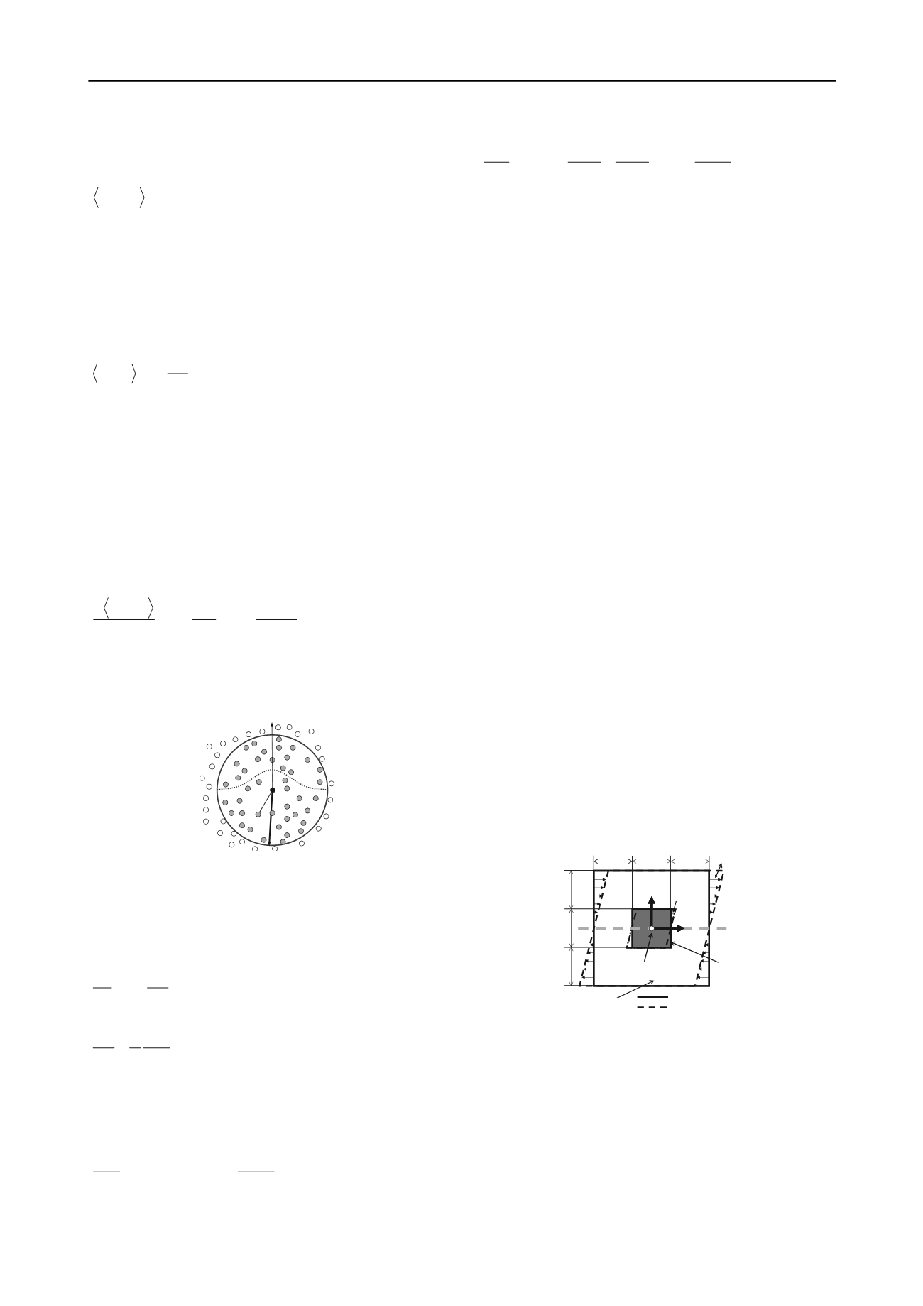
3 SIMULATION OF SIMPLE SHEAR TEST
In the validations of the SPH method for solid mechanics, a
simulation of simple shear test under plane strain condition is
carried out using Drucker-Prager model and Super-subloading
Yield Surface Modified Cam-clay model. Calculated stress
strain relation and stress paths are compared with the theoretical
solution at the center of specimen. Figure 2 illustrates the
numerical model used in the simulation. As the figure indicates,
the specimen is a square object (10 cm by 10 cm). In the SPH
method, numerical instabilities and errors tend to arise due to
lack of calculation points. Therefore, a virtual area surrounded
the specimen was used in this simulation. The solid line denotes
the initial configuration of the specimen, and the dashed line
denotes the configuration after deformation. In the simulation,
the virtual area is forcibly deformed with a constant
displacement to represent simple shear conditions, and the
deformation of the specimen is calculated. Since a virtual area
surrounded the specimen, only the scheme is employed in this
validation. The parameters used in this simulation are
summarized in Tables 1. As Table 1 indicates, seven different
cases are considered in this simulation. In Cases 1, cohesive
frictional material is used. In Cases 2 and 3, parameters of
typical clay under two different values of the initial mean stress
and initial overconsolidation ratio are used. In Cases 4 to 7,
parameters of typical sand under three different values of the
initial mean stress and degree of structure are utilized.
before deformation
after deformation
virtual area
L
L
L
L
center axis
L
L
L=10cm
specimen
v
x
measurement point
for stress and strain
y
x
xy
Figure 2. Numerical model
Figures 3 to 5 shows calculated stress-strain relation and
stress paths at the center of the specimen. The theoretical
solutions are also described in these figures for comparison. The
solid line denotes the theoretical solutions, and plotted points
indicate the obtained results. Based on the comparison, the
results from the SPH scheme are in good agreement with the
theoretical solution. Also, by introducing the Super-subloading
Yield Surface Modified Cam-clay model (Asaoka et al. 2000;
2002) into the method, the softening with plastic compression
behavior of structured soil and rewinding behavior of
overconsolidated clay (Fig. 4) are expressed. Also, the softening
behaviors with plastic compression of medium-dense sand and
subsequent hardening behavior with plastic expansion (Fig. 5)


