2222
Proceedings of the 18
th
International Conference on Soil Mechanics and Geotechnical Engineering, Paris 2013
In this case, as both
M
and
D
are the parents of
S
,
S
is the
parent of
L
, and both
S
and
L
are the parents of
B
, the joint
probability can be derived according to Eq. 2:
P(B = B
1
, M = M
i
, D = D
j
, S = S
k
, L = L
m
)
= P(M = M
i
)× P(D = D
j
)× P(S = S
k
|
M = M
i
, D = D
j
)
× P(L = L
m
|
S = S
k
) × P(B = B
1
|
S = S
k
, L = L
m
)
(4)
where the (conditional) probabilities on the right hand side of
the equation are quantified with available information (e.g., sta-
tistical data, expert knowledge, and physical approaches).
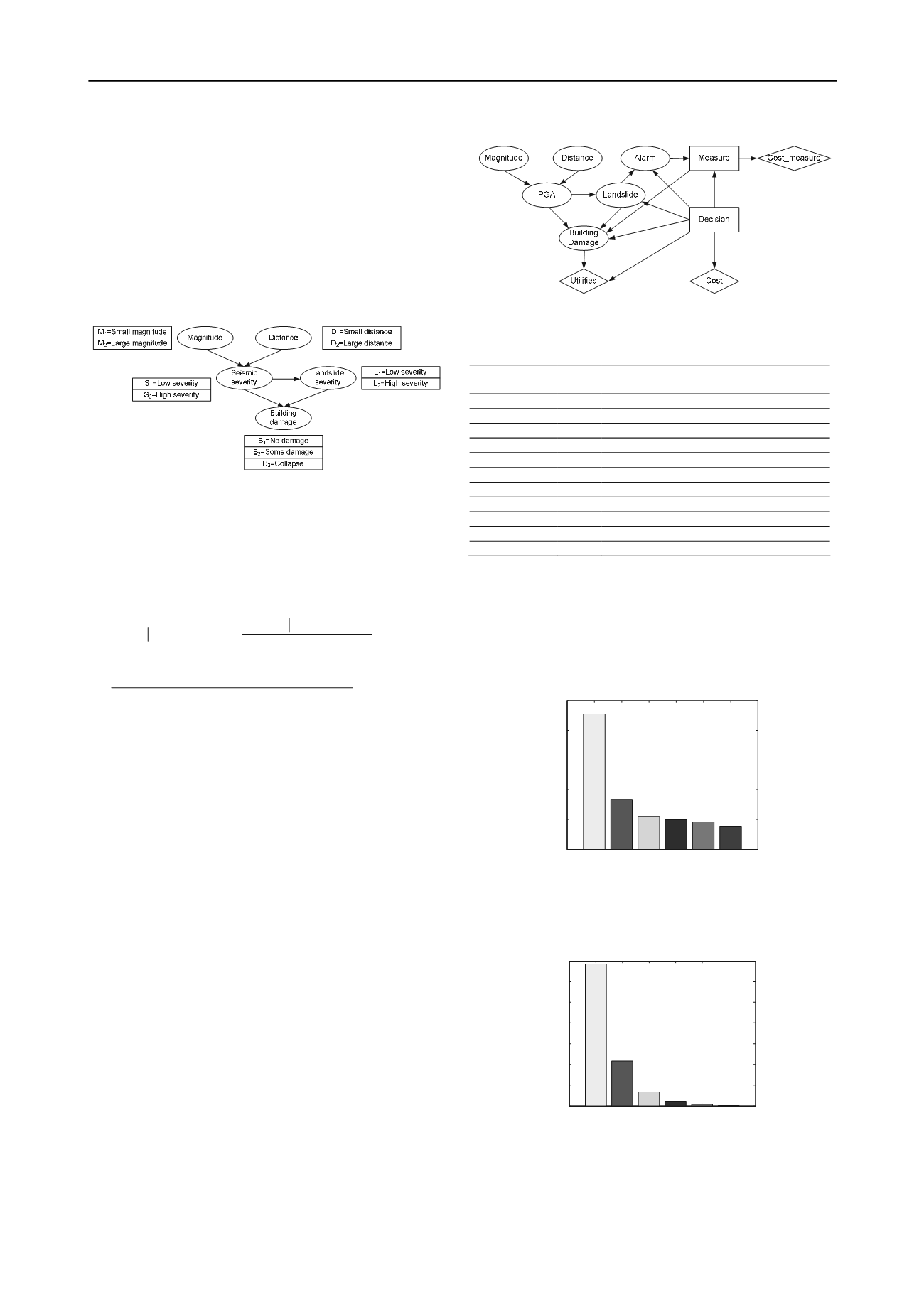
Fig. 1 A simple Bayesian network.
The BN allows one to enter evidence as input, meaning that
probabilities in the network are updated when new information
is made available, for instance, a case with a small magnitude
and large distance. This information will propagate through the
network and the posterior probabilities of
B, P(B = B
1
)
can be
calculated as:
1
1
2
1
1
2
1
2
2 2
1
1
2
1 1
3 2 2
1
2
1 1 1
,
,
,
,
,
,
,
,
,
,
,
j
i
j
i
k
j
i
k j
i
P B B M M D D
P B B M M D D
P M M D D
P B B S S L L M M D D
P B B S S L L M M D D
(5)
where the joint probabilities in the above equation are calcu-
lated with Eq. 3 on
the basis of Baye’s
theorem (Ang and Tang
2007).
3 BAYESIAN NETWORK FOR EARTHQUAKE-
TRIGGERED LANDSLIDE RISK ASSESSMENT
According to the ISSMGE Glossary of Risk Assessment Terms,
‘Risk’ is the measure of the probability and severity of an a
d-
verse effect to life, health, property, or the environment. Quanti-
tatively risk is the product of the threat times the potential worth
of loss and can be expressed as:
Risk = Probability of Threat×Worth of Loss
(6)
Otherwise expressed (e.g. Einstein 1997):
Risk = P(T)× P(E|T) × U(E)
(7)
where
P(T)
is probability of threat,
P(E|T)
is conditional prob-
ability of damage of the element(s) at risk exposed to threat, i.e.
vulnerability, and
U(E)
is utility of element(s) at risk.
A comprehensive Bayesian network (modified after Einstein
et al
2010) for estimating the risk of buildings in an assumed
earthquake-triggered landslide case was built with an open-
source MATLAB package BNT (Bayes Net Toolbox) (Murphy
2001) as shown in Fig. 2. There are 11 nodes and 16 arcs in the
network. Each node is characterized by several discrete states as
shown in Table 1.
Fig. 2 Bayesian network for earthquake-triggered landslide risk assess-
ment with possible decisions (modified after Einstein
et al
2010).
Table 1 Nodes and their states of the Bayesian network in Fig. 2
Nodes
No. of
states
States
Magnitude (M
w
)
6
4.0-4.5-5.0-5.5-6.0-6.5-7.0
Distance (km)
6
22-25-28-31-34-37-40
PGA (g)
6
0-0.08-0.16-0.24-0.32-0.40-0.48
Landslide
2
Happens; Does not
Building damage 3
No damage; Some damage; Collapse
Alarm
2
Yes; No
Measure
2
Yes; No
Decision
4 Passive; Active; No action; Warning system
Cost_measure
-
Cost
-
Utilities
-
4 QUANTIFYING THE NETWORK
4.1
Seismic hazard
The seismic source is assumed as a line source in this study. Us-
ing the geometric characteristics of the source, the distribution
of distances can be calculated as shown in Fig. 3.
22-25 25-28 28-31 31-34 34-37 37-40
0
0.1
0.2
0.3
0.4
0.5
Distance/km
Probability
Fig. 3 Specification of the discrete probabilities of distance.
The annual probabilities for each range of Mw are calculated
using the Gutenberg-Richter magnitude recurrence relationship
(Gutenberg and Richter 1994), as shown in Fig. 4.
4.0-4.5 4.5-5.0 5.0-5.5 5.5-6.0 6.0-6.5 6.5-7.0
0
0.1
0.2
0.3
0.4
0.5
0.6
0.7
Magnitude, Mw
Probability
Fig. 4 Specification of the discrete probabilities of magnitude.
The conditional probabilities of PGA given the magnitude
and distance to epicenter are calculated with the ground motion
equation proposed by Ambraseys
et al
(2005), using Monte
Carlo simulation in Microsoft Excel. The joint probabilities of


