2219
Technical Committee 208 /
Comité technique 208
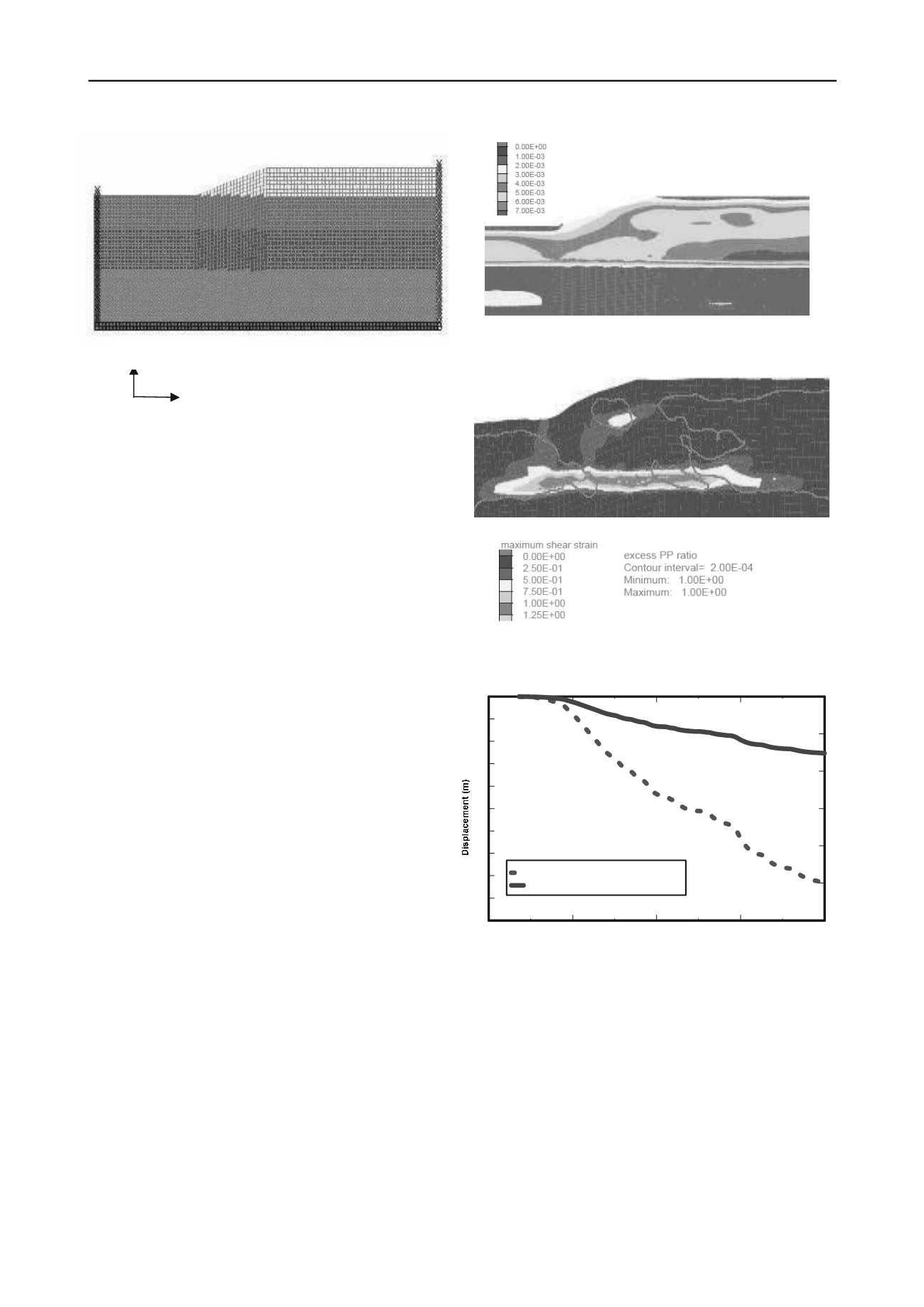
Figure 4. FLAC model for the modeling
The static equilibrium state at the time of the earthquake event
is established to obtain the initial shear-stress distribution of the
soil mass.
The preliminary analysis, assuming undamped
elastic-material, was performed to estimate maximum levels of
cyclic shear strains and velocity levels throughout the model
during the dynamic excitation. The maximum shear strain
contour from the preliminary run is shown on Figure 5
indicating that the maximum elastic shear strains are smaller
than 0.7 % throughout almost the entire modeled area. This
range of shear strains is considered appropriate for inclusion of
hysteretic damping based upon the dynamic characteristics of
the soils as illustrated on Figure 2. The frequency range for the
natural response of the elastic materials is calculated to be
relatively uniform throughout the model, with a dominant
frequency of approximately 3 Hz.
A fully coupled nonlinear seismic analysis is performed using
the Mohr-Coulomb model to represent the soil layers, with
additional hysteretic damping applied to simulate the
non-linear soil dynamic behavior. Due to the fact that hysteretic
damping does not completely damp high frequency component,
a small amount of stiffness-proportional Rayleigh damping is
also employed in the analysis.
The Finn-Byrne model is used for the liquefaction simulation by
considering Strata I and II as liquefiable materials. Based on
CPT/SPT correlations from in-situ CPT data and fine contents
(Kulhawy and Mayne, 1990), the equivalent normalized SPT
blow counts are assigned for the two strata. The automatic
rezoning logic is applied in the analysis to correct for severely
distorted mesh conditions developed during the simulation of
earthquake shaking. The onset of liquefaction is identified by
the cyclic pore-pressure ratio, u
e
/
c
’
, where u
e
is the excess pore
pressure and
c
’is the initial
in-situ effective confining pressure.
After the liquefaction, the soil shear strength is reduced to
residual strength which is 30% of the original value.
The numerical analysis indicates the development of
liquefaction and failure surface in the slope. Figure 6 displays
the contours of maximum shear strain at the end of earthquake
excitation (40 seconds). The contour of excess pore pressure
ratio equaling 1 (onset of liquefaction) at 40 seconds is also
marked in green line on Figure 6. Figure 7 shows the vertical
and horizontal displacement histories at the slope crest. The
negative sign for X and Y axes indicate the left direction and
downward direction, respectively. the slope moves horizontally
approximately 8.5m.
Figure 5. Maximum shear strain contours from undamped elastic
analysis
Figure 6. Shear strain contours and excess pore pressure ratio=1 contour
at 40 seconds
Figure 7. Horizontal (x) and vertical (y) displacement histories at crest
of the slope
3 DEBRIS FLOW RUN-OUT DISTANCE
After the development of liquefaction and failure surface in the
slope, debris flow can be triggered and the remolded mass
during initial failure travels further downslope until the initial
stored potential energy is dissipated by friction.
The debris flow run-out distance can be estimated using one- or
two- dimensional numerical modeling of sediment-laden
submarine flow. For this study, the one-dimensional (1-D)
model
BING
assuming one phase flow and
“constant volume”
constraint. The required input for the simulation includes the
bed profile over which the debris mass flow, the initial
configuration of the pile of debris slurry, rheological parameters
describing the debris slurry and numerical parameters to
describe spatial and temporal discretization, run duration and
X (Horizontal) Displacement (Left)
Y(Vertical) Displacement (Downward)
X, horizontal distance
Y, height


