1775
Technical Committee 204 /
Comité technique 204
Settlement (mm)
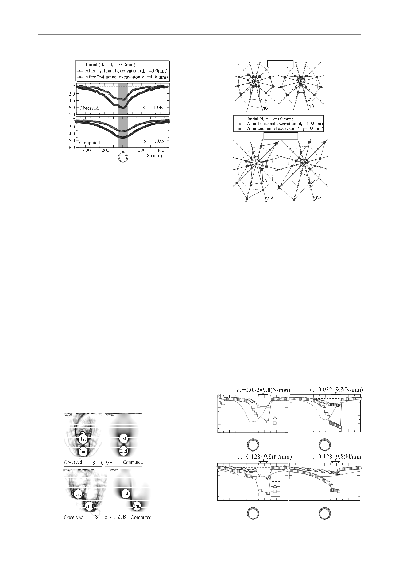
Figure 6. Surface settlement profile
–
vertically downward
Figure 7 shows the distributions of obseved and computed
shear strain. The distribution of shear strain of the model tests
are obtained from the simulation of Particle Image Velocimetry
(PIV) technique. The figures show the results of the cases where
the following tunnel is situated directly underneath (S
T1
=0.25B)
and diagonally downward (S
T1
=S
T2
=0.25B). The concentration
of the strain is represented with the color contrast indicated in
the legend. It is seen in the result that the shear band of the
ground is developed from the tunnel invert and covered the
entire tunnel during tunnel excavation. It is also seen that shear
strain occurs towards the preceding tunnel due to the excavation
of the following tunnel. A region of large strain concentration is
seen in between the twin tunnels due to excavation of the
following tunnel for both S
T1
=0.25B and S
T1
=S
T2
=0.25B.The
shear strain of the numerical analyses shows very good
agreement with the results of the model tests.
Figure 8 shows the observed and computed earth pressure
distributions for
D/B
=2.0 where the following tunnel is situated
directly underneath (S
T1
=0.25B) and diagonally downward
(S
T1
=S
T2
=0.25B). It is seen that in S
T1
=0.25B (directly
underneath) for the excavation of the preceding (1
st
) tunnel
earth pressure decreases around this tunnel due to the arching
effect, the same as the results of the references (Murayama and
Matsuoka, 1971; Adachi et al., 1994; Shahin et al. 2004 &
2011). As shear band develops surrounding the tunnel (Fig.7)
the surrounding ground undergoes to a loosen state which
reduces stresses in that place. However, the earth pressure at
both side of the tunnel increases and it decreases at the tunnel
invert during excavation of the following tunnel. On the other
hand, when the following tunnel is constructed at
S
T1
=S
T2
=0.25B (diagonally downward), earth pressure of the
preceding tunnel increases at the right shoulder and the left part
of the tunnel invert. The numerical analyses perfectly capture
the distributions of earth pressure for the excavation of the
following tunnel in two different locations.
Figure 8. Earth pressure distribution at the preceding tunnel after the
excavation of the following tunnel
4.2
Tunnel excavation considering building loads
Figure 9(a) shows the observed and computed surface
settlements profiles for 1mm and 4mm of shrinkage in
D/B
=1.0
(shallow tunneling) where strip foundation is used to consider
building loads. Figure 9(b) shows the observed and computed
surface settlements profiles for
D/B
=4.0 (tunneling in deep
underground) where pile foundation is used to consider building
loads. Here, the distance between the crown of tunnel and the
pile tip is 10cm (10m in prototype scale). These figures also
represent the results of the green field condition for the
shrinkage of
d
r
=4mm, which is shown with solid line. The
position of the applied dead load and the position of tunnel are
depicted at the top and the bottom in the figure, respectively. It
is seen that the maximum surface settlement occurs at the
position of the building load as observed in the previous
researches (Shahin et al., 2004 & 2011). The deep underground
tunneling has a significant effect on the existing structure. The
numerical simulations can explain well the results of the model
tests. It is also noticed that surface settlement troughs for tunnel
excavation in the ground disturbed by existing buildings do not
follow the usual pattern of a Gaussian distribution curve even in
the deep tunneling, as observed for the Greenfield condition.
-200 -100 0 100 200 300
x(mm)
(b)computed
-300 -200 -100 0 100 200
0
2
4
6
8
Settlement (mm)
x(mm)
(a) observed
D/B
=4.0
Initial (d
r
=0.0mm)
d
r
=1.0mm
d
r
=4.0mm
d
r
=4.0mm(Greenfield)
-300 -200 -100 0 100 200
0
2
4
6
8
Settlement(mm)
x(mm)
D/B
=1.0
-200 -100 0 100 200 300
x(mm)
Initial (d
r
=0.0mm)
d
r
=1.0mm
d
r
=4.0mm
d
r
=4.0mm(Greenfield)
(a) Observed
(b) Computed
(b) pile foundation
Figure 9. Surface settlement profiles
(a) Observed
(b) Computed
S
T1
=0.25B
S
T1
=S
T2
=0.25B
B
n
(
×
98kPa)
n
(
×
98kPa)
(a) strip foundation
Figure 7. Strain distribution in the ground


