1408
Proceedings of the 18
th
International Conference on Soil Mechanics and Geotechnical Engineering, Paris 2013
models was measured using accelerometers and laser
displacement transducers installed on the slope models.
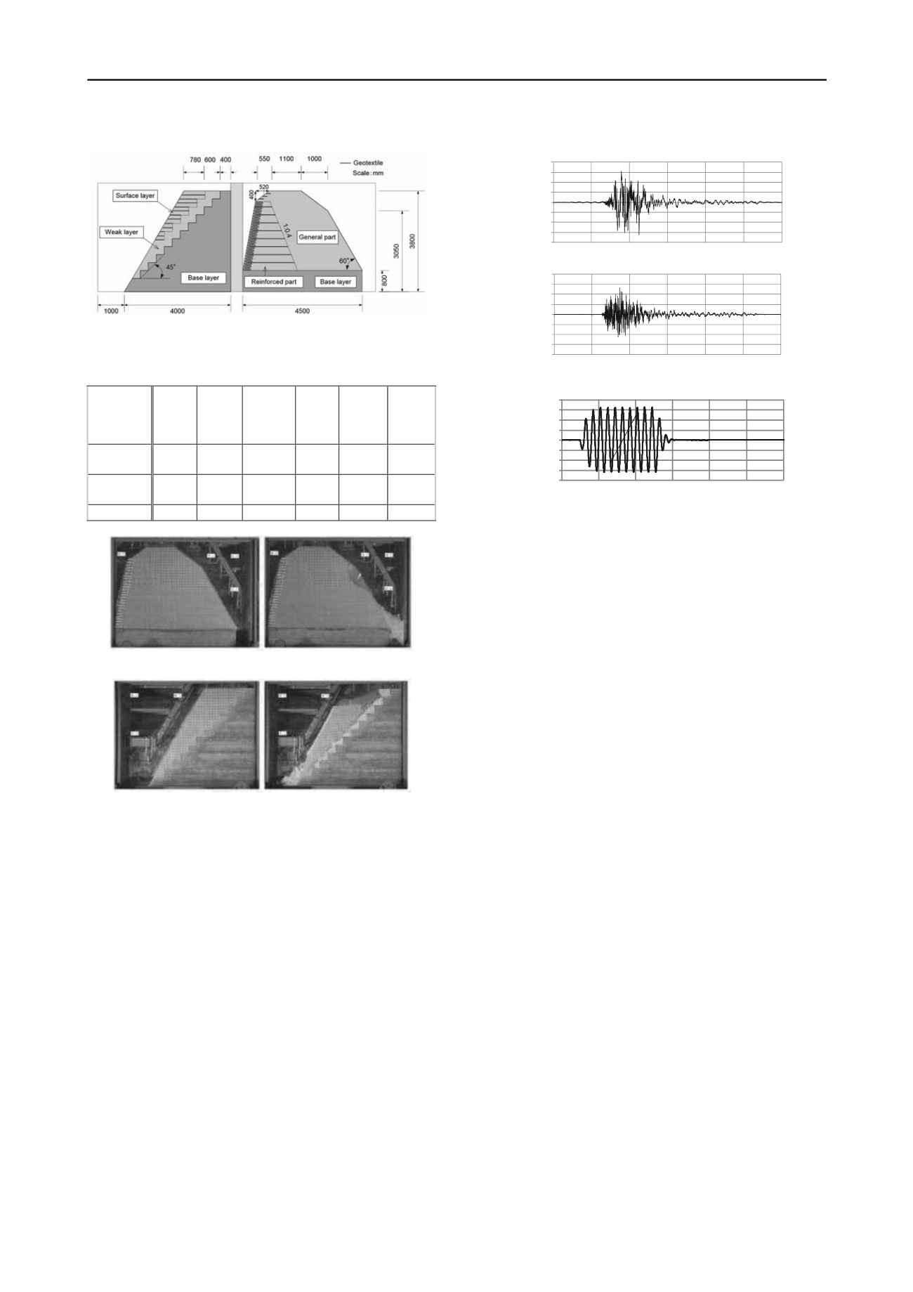
Figure 1. Initial state of test models (left figure: three layered model,
right figure: one layered model)
Table 1. Slope model soil properties as determined from tri-axial
compression tests with the materials in the layers
Young’s
modulus
(kN/m
2
)
Initial
shear
modulus
(kN/m
2
)
The input waves in the shaking table tests were a 5 Hz sine
wave with a wave number of 10 and an observed seismic wave
in Niigata Chuetsu earthquake in 2007 (dominant frequency: 0.5
Hz). The amplitude of the waves was increased in stepwise
changes with 50 to 100 gal pace. The waves were input along
lateral and vertical directions on the condition that amplitude of
vertical wave was two thirds of that of lateral one.
Figure 2 shows the initial and final photos of test models. The
one layered model exhibited partial catastrophic failure at right
hand side slope when the input wave amplitude reached 654 gal
for lateral wave and 537 gal for vertical wave of the observed
seismic wave shown in Figure 3 (a). The three layered model
exhibited slide down along the slip surface generated in the
weak layer when the input wave amplitude reached 984 gal for
lateral wave of the sine wave shown in Figure 3 (b). These
waves are used as input waves in below-mentioned analyses.
3 ANALYTICAL METHOD
-800
-600
-400
-200
0
200
400
600
800
0.0
10.0
20.0
30.0
40.0
50.0
60.0
Input lateral acceleration
(
gal
)
Time (sec)
-800
-600
-400
-200
0
200
400
600
800
0.0
10.0
20.0
30.0
40.0
50.0
60.0
I nputvertical acceleration
(
gal
)
Time (sec)
(a) Input waves for one layered model
-1,200
-900
-600
-300
0
300
600
900
1,200
0.0
1.0
2.0
3.0
4.0
5.0
6.0
3.1
FEM
FEM analysis was carried out focusing on the investigation of
possibility of analyzing the amplification and phase lag of
response acceleration at the top of slope of the one layered
model. The GHE-S model (Murono and Nogami, 2006)
together with the multiple nonlinear spring model (Towhata and
Ishihara, 1985) was used as a constitutive law of the general and
reinforced part. Considering confining pressure dependency of
initial shear modulus
G
0
, relationship between
G
/
G
0
(
G
: shear
modulus) and damping ratio
h
and shear strain
γ
are modeled by
the GHE-S model as shown in Figure 4. Elasticity model was
used as a constitutive law of the base layer. Wave attenuation
was considered by Rayleigh damping (damping constants α =
0.0 and β = 0.001).
3.2
MPM
The MPM (Sulsky et al, 1994 and 1995), which is one of the
mesh-free methods, was used as the analytical method. Figure 5
explains analysis flow of the MPM, which is similar to that of
FLAC (Cundall and Board, 1988). But, the MPM can deal with
larger deformation through particle discretization. The MPM
also avoids tensile instability that is annoying in the Smoothed
Particle Hydrodynamics (SPH) (Lucy, 1977; Gingold and
Monaghan, 1977). Hence, the MPM does not need an artificial
damping. The super/subloading yield surface (SYS) Cam-clay
model (Asaoka et al, 2000) was used as an elasto-plastic
constitutive law for general part and weak layer in the MPM
model. The model can describe degradation processes from both
an overconsolidated state to a normally consolidated state and
from a structured state to a destructured state. Figure 6 shows
the results of investigation to determine the stress-strain
characteristics of a material specimen in the general part and
weak layer under tri-axial compression tests and cyclic tri-axial
tests using the model with the parameters shown in Table 2. On
the other hand, the perfect elasto-plastic Drucker-Prager model
and the elasticity model were used for the surface layer of three
layered model and base layers as a constitutive law,
respectively.
Poisson’s
ratio
Unit
weight
(kN/m
3
)
Cohesion
(kN/m
2
)
Internal
frictional
angle
(deg)
General part
Weak layer 7.7×10
4
2.9×10
4
Inputlateralacceleration
�i
gal
�j
sec)
Time (
(b) Input wave for three layered model
Figure 3. Input waves used in FEM and MPM anaysis
0.264
16.2
12.9
24.6
Reinforced
part
9.4×10
4
3.5×10
4
0.383
16.2
17.6
19.4
Base layer 2.5×10
6
9.4×10
5
0.267
18.5
280.5
57.3
(a) One layered model
(b) Three layered model
Figure 2. Initial and final photos of test models (above figure: one
layered model, below figure: three layered model)


