728
Proceedings of the 18
th
International Conference on Soil Mechanics and Geotechnical Engineering, Paris 2013
indefinite value. It has been proposed an analysis method using
the constrained condition to restrict a magnitude of
displacement velocity in the ultimate bearing capacity problems.
But, it can not apply the constrained condition in the
deformation analysis. Therefore, we defined the magnitude of
displacement velocity using the equation of motion (using the
momentum) in this study.
The equation (6) is the equation of motion at the reference
configuration. Here,
,
,
is a mass, an acceleration, a
nominal stress at the reference configuration.
g
is a gravitational
acceleration.
u
0
0
Div
π g
u
(6)
It is obtained a weak form by to apply the principle of virtual
work to the equation of motion (6). In addition, it is obtained
the equation (7) as a weak form of equation of motion by to
update to the current configuration from the reference
configuration besed on the updated lagrange method. Here,
V,
S
is a volume boundary, a sress boundary at the current
configuration.
,
is a mass, a ttrue stress at the current
configuration.
:
V
V
S
V
div dV
dV
dS
dV
σ u
u u
t u
g u
(7)
As shown in the equation (5), the rigid plastic constitutive
equation has characteristic that the true stress is decided from
the boundary problems at the current configuration because
there are not effect by the stress history. The rigid plastic
dynamic deformation analysis is formulated as shown in the
equation (8) by to apply the rigid plastic constitutive equation to
the equation (7). Here, it need to repetition calculation because
the equation (8) is the nonlinear equation having a acceleration
(displacement acceleration), a displacement velocity and a
displacement. Therefore, we carried out analysis by the direct
substitution method in this study. In addition, the proposed
method applied the implicit method by the wilson’ s
method
because the equation (8) has the acceleration (displacement
acceleration) and the displacement velocity of unknown.
2
2
:
3 +1 2
3
:
3 +1 2
V
v
V
S
V
V
div dV
e
e
d
e
dS
dV
dV
for
iv dV
ε
u
ε
I
u
t u
g u
u u
u
(8)
The equation of motion expresses dynamic behavior of the
ground against action force. There is a characteristic that an
equilibrium of disagreement between the external load and the
internal stress by the inertia force is satisfied from viewpoint of
the static equilibrium equation. Therefore it can keep the
equilibrium by the inertia force against the external load of if
the ground can not bear. However, there is a possibility to occur
sudden deformation because of large acceleration (displacement
acceleration) due to the inertia force. Therefore, it is expressed
the velocity effect of bearing capacity with dynamic behavior
by the inertia force even if the ground's strength is constant.
3 VERIFICATION OF ANALYSIS METHOD
This chapter will show result of the limit bearing capacity
analysis and the dynamic deformation analysis against the
analysis condition at the Table 1 and the horizontal ground
model at the Figure 1. This calculation does not consider the
body force. And, it does not update coordinate from the
reference configuration based on the infinitesimal deformation
theory to compare to the theoretical solution.
The Prandtl has shown the theoretical solution
( )
2
c
+
in the
limit bearing capacity of the horizontal ground. The theoretical
solution of the limit bearing capacity is obtained 102.83 kPa
from the Table 1.
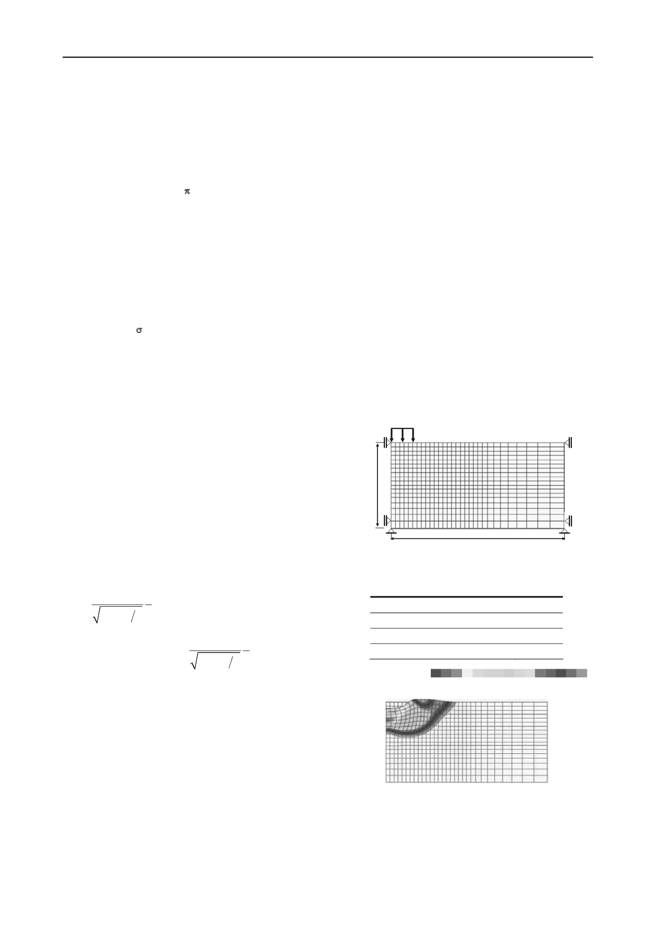
Next, we show the equivalence strain velocity distribution and
the collapse mode of the ground at the Figure 2 as result of the
limit bearing capacity analysis using the rigid plastic
constitutive equation (5). The collapse mode expresses by to use
a displacement which multiplied a displacement velocity to any
time. It showed that has been obtained similar collapse mode
when compared to the Prandtl’s theoretical collapse mode.
In addition, this analysis obtained 104.87 kPa as the limit
bearing capacity.
Next, we show the result (a relationship of the loading and the
displacement acceleration, the displacement velocity, the
displacement) of the dynamic deformation analysis used the
rigid plastic constitutive equation (5) of the proposed method at
the Figure 3. We applied a loading velocity of 10.0 kPa/sec (a
time interval
t of 0.1 sec/step) as the analysis condition. It is
30.0
15.0
0
F
Figure 1. Analysis model [Length unit : m]
Table 1. Analysis condition
Angle of shear resistance
[°]
0.0
Cohesion
c
[kPa]
20.0
Unit weight
γ
t
[kN/m
3
]
0.0
Initial loading
F
0
[
kPa
]
20.0
max
e
min
e
Figure 2. The collapse mode and the equivalence strain velocity
distribution by the limit bearing capacity analysis (the limit bearing
capacity is 104.87 kPa)


