733
Technical Committee 103 /
Comité technique 103
5 RANDOM FINITE ELEMENT LIMIT ANALYSIS
The RFLA involves the generation and mapping of a random
field of properties onto a finite element mesh. Full account is
taken of local averaging and variance reduction over elements,
and an exponentially decaying (Markov) spatial correlation
function is incorporated. To be consistent with local averaging
procedure, four linear triangluar elements within a square area
were assigned a constant property in both lower and upper
bound analysis. It should be mentioned that random properties
are also assigned to the kinematically admissible discontinuities
involved in upper bound analysis. The analysis is repeated
numerous times using Monte-Carlo simulations. Each
realization of the Monte-Carlo process involves the same
underlying mean, standard deviation and spatial correlation
length of soil properties, however the spatial distribution of
properties varies from one realization to the next. Following a
suite of Monte-carlo simulations, the mean and coefficient of
variation of the bearing capacity factor can be easily estimated.
Figure 2 shows a typical deformed mesh at failure by lower
bound limit analysis with a superimposed greyscale
corresponding to
1
u
c
, in which lighter regions indicated
weaker soil and darker regions indicated stronger soil. In this
case the dark zones and the light zones are roughly the width of
the footing itself, and it appears that the weak (light) region near
the ground surface to the left of the footing has triggered a quite
non-symmetric failure mechanism.
Figure 3 compares RFLA and RFEM for ten typical
simulations. It can be seen from Figure 2 that the RFEM is
always bounded by the RFLA results.
Figure 2. Typical deformed mesh and greyscale at failure with
1
u
c
. (the darker zones indicate stronger soil)
5
10
2.0
2.5
3.0
3.5
4.0
4.5
5.0
5.5
6.0
N
c
Realization
FEM
LB
UB
Figure 3. Comparison of lower and upper bounds with finite
element analysis for ten typical simulations.
6 PROBABILISTIC ANALYSES
Analyses were performed using the input parameters in the
range
0.125
4
u
c
and
0.125
4
u
c
V
. For each combination
of
u
c
and
u
c
V
, 1000 realizations of the Monte Carlo process
were performed, and the estimated mean and standard deviation
of the resulting 1000 bearing capacity factors were computed.
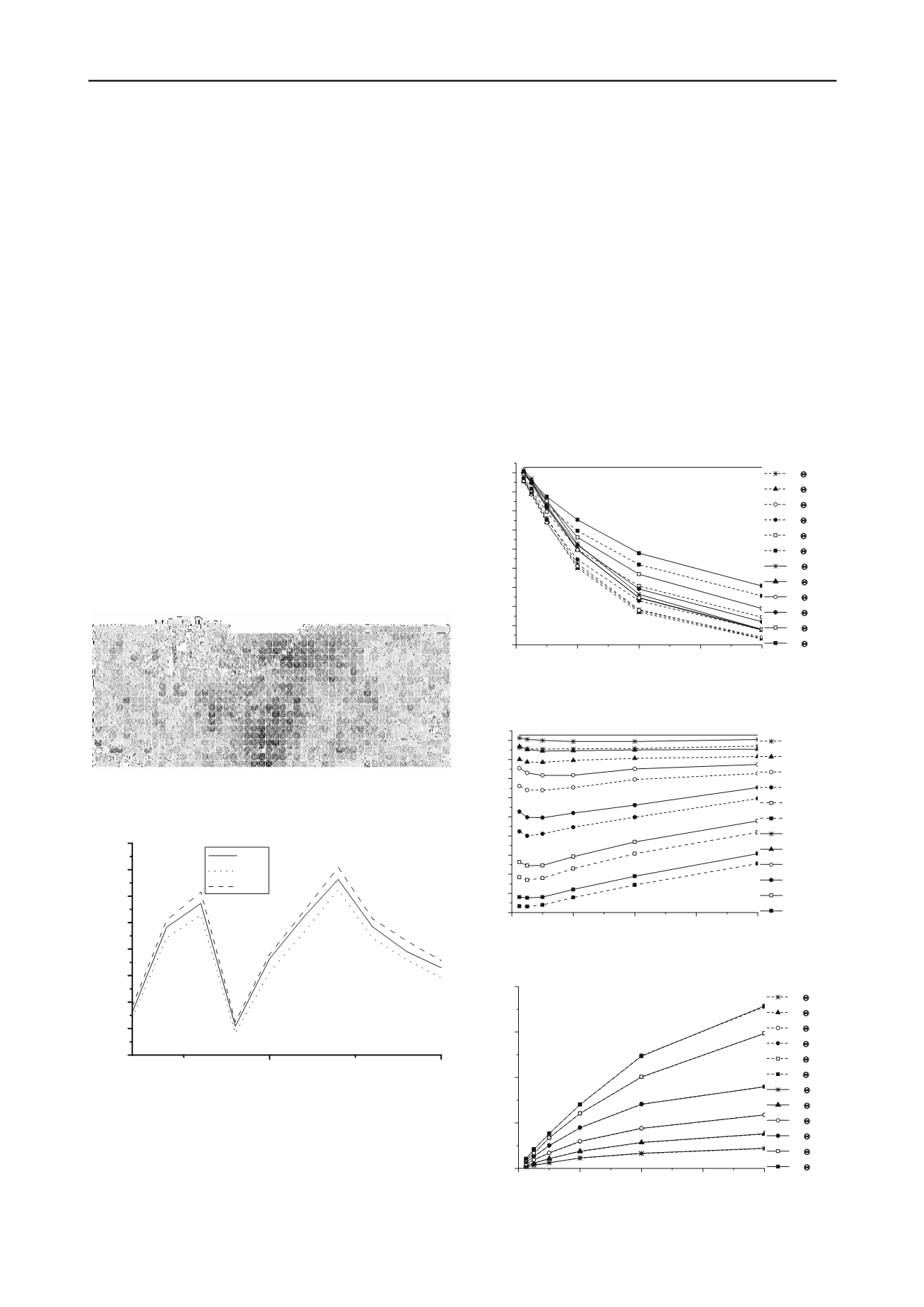
Figure 4 shows how the estimated mean bearing capacity factor,
l
N
and
u
N
, varies with
u
c
and
u
c
V
(The RFEM results were
omitted due to length limit). The plot confirms that, for low
values of
u
c
V
,
l
N
and
u
N
tend to the deterministic Prandtl
value of 5.14. For higher values of
u
c
V
, however, the mean
bearing capacity factors fall steeply, especially for lower values
of
u
c
.What this implies from a design standpoint is that the
bearing capacity of a heterogeneous soil will on average be less
than the Prandtl solution that would be predicted assuming the
soil is homogeneous with its strength given by the mean value.
The influence of
u
c
is also pronounced with the greatest
reduction from the Prandtl solution being observed with values
around
0.5
u
c
. Figure 6 shows the influence of
u
c
and
u
c
V
on the estimated coefficient of variation of the bearing capacity
factor . The plots indicate that
l
N
and
u
N
are positively
correlated with both
u
c
and
u
c
V
. It is also interesting to note
that there are essential no difference between
l
N
V
and
u
N
V
.
Figure 4. Estimated mean bearing capacity factors
l
N
and
u
N
verse the coefficient of variation of undrained shear strength
Figure 5. Estimated mean bearing capacity factors
l
N
and
u
N
verse the spatial correlation length of undrained shear strength
Figure 6. Estimated coefficient of variation of the bearing
capacity factors
l
N
and
u
N
0.0
1.0
2.0
3.0
4.0
0.5
1.0
1.5
2.0
2.5
3.0
3.5
4.0
4.5
5.0
LB,
Vc
u
=0.125
LB,
Vc
u
=0.25
LB,
Vc
u
=0.5
LB,
Vc
u
=1.0
LB,
Vc
u
=2.0
LB,
Vc
u
=4.0
UB,
Vc
u
=0.125
UB,
Vc
u
=0.25
UB,
Vc
u
=0.5
UB,
Vc
u
=1.0
UB,
Vc
u
=2.0
UB,
Vc
u
=4.0
c
c
u
Prandtl, 5.14
0.0
1.0
2.0
3.0
4.0
0.0
0.5
1.0
1.5
2.0
LB,
c
u
=0.125
LB,
c
u
=0.25
LB,
c
u
=0.5
LB,
c
u
=1.0
LB,
c
u
=2.0
LB,
c
u
=4.0
UB,
c
u
=0.125
UB,
c
u
=0.25
UB,
c
u
=0.5
UB,
c
u
=1.0
UB,
c
u
=2.0
UB,
c
u
=4.0
V
c
V
c
u
0.0
1.0
2.0
3.0
4.0
0.5
1.0
1.5
2.0
2.5
3.0
3.5
4.0
4.5
5.0
LB,
c
u
=0.125
LB,
c
u
=0.25
LB,
c
u
=0.5
LB,
c
u
=1.0
LB,
c
u
=2.0
LB,
c
u
=4.0
UB,
c
u
=0.125
UB,
c
u
=0.25
UB,
c
u
=0.5
UB,
c
u
=1.0
UB,
c
u
=2.0
UB,
c
u
=4.0
c
V
c
u
Prandtl, 5.14


