732
Proceedings of the 18
th
International Conference on Soil Mechanics and Geotechnical Engineering, Paris 2013
(1)
where
A
is an equilibrium matrix,
σ
is a vector containing
stresses, and the external load consists of a constant part
0
p
and
a part proportional to a scalar parameter
,
f
defines the yield
conditions.
A statically admissible stress field is one which satisfies (a)
the stress boundary conditions, (b) equilibrium, and (c) the yield
condition (the stresses must lie inside or on the yield surface in
stress space).
The upper bound theorem states that the load (or the load
multiplier), determined by equating the internal power
dissipation to the power expended by the external loads in a
kinematically admissible velocity field, is not less than the
actual collapse load. Based on the duality between the upper
and lower bound methods, Krabbenholf et. al (2005) derived a
upper bound formulation in terms of stresses rather than
velocities and plastic multipliers. This allows for a much
simpler implementation and general nonlinear yield conditions
can be easily dealt with.
T
0
maximize
subject to
=
( ) 0
B
σ
p p
f
σ
(2)
where
=
A
B LN
and
A
is the area of elements,
N
contains
the interpolation functions and
L
is defined as (for linear
triangular elements)
T
/
0 /
0 /
/
x
y
y
x
L
It should be mentioned that matrix
B
in Eq. (2) can be
amended to include kinematically admissible discontinuities,
which have previously been shown to be very efficient (e.g.,
Sloan and Kleeman 1995).
Although both upper and lower bound methods formulated
as Eqs. (1) and (2) with a Tresca failure criterion are ready to be
solved by public available second order cone programming
packages (e.g., SeDumi, Mosek), our in-house limit analysis
program (Lyamin and Sloan 2002a and 2002b) is used in this
study.
3 DETERMINISTIC ANALYSES
The bearing capacity analyses use an elastic-perfectly plastic
stress-strain law with a Tresca failure criterion. Triangular
constant stress
–
linear velocity element is used for both upper
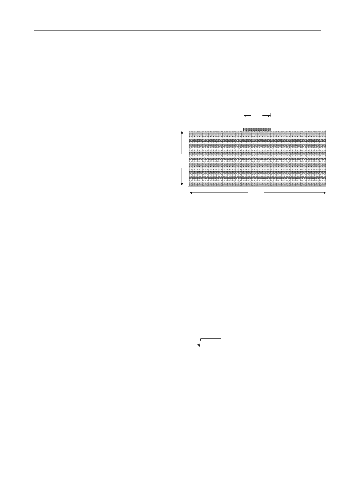
and lower bound analysis in this study. A mesh is shown in Fig.
1 consisting of 4000 triangular elements. The strip footing has a
width of 10 elements. The bottom of the mesh while the sides
are allowed to move only in the vertical direction. Plastic stress
redistribution in RFEM analysis is accomplished using a
viscoplastic algorithm. For RFEM analysis, 8-node quadrilateral
elements and reduced Gaussian integration in both the stiffness
and stress redistribution parts of the algorithm (Smith and
Griffiths 2004). The mesh for RFEM analysis is not shown but
one can easily figure it out by treating four triangular elements
as a square 8-node quadrilateral element.
Rather than deal with the actual bearing capacity, this study
focuses on the dimensionless bearing capacity factor
c
N
,
defined as
f
c
u
q
N
c
(3)
where
f
q
is the bearing capacity and
u
c
is the undrained shear
strength of the soil beneath the footing. For a homogeneous soil
with a constant undrained shear strength,
c
N
is given by the
Prandtl solution, and equals
2
or 5.14.
The lower bound and upper bound bearing capacity factor
are found to be 5.02 and 5.19 respectively. The bearing capacity
factor obtained by FEM analysis is 5.12. Although the FEM
result lies in between the lower and upper bound bearing
capacity factors, it lacks error estimation on the limit load.
Figure 1. Finite element mesh for limit analysis
4 PROBABILISTIC DESCRIPTIONS OF STRENGTH
PARAMETERS
In this study, the dimensionless shear strength parameter
u
c
is
assumed to be a random variable characterized statistically by a
lognormal distribution (i.e. the logarithm of the property is
normally distributed). The lognormally distributed shear
strength
u
c
has three parameters; the mean,
u
c
, the standard
deviation
u
c
and the spatial correlation length
ln
u
c
. The
variability of
u
c
can conveniently be expressed by the
dimensionless coefficient of variation defined as
u
u
u
c
c
c
V
(4)
The parameters of the normal distribution (of the logarithm
of
u
c
) can be obtained from the standard deviation and mean of
u
c
as follows:
2
ln
ln 1
u
u
c
c
V
(5)
2
ln
ln
1
ln
2
u
u
u
c
c
c
(6)
A third parameter, the spatial correlation length
ln
u
c
, will
also be considered in this study. Since the actual undrained
shear strength field is assumed to be lognormally distributed, its
logarithm yields an “underlying” normal distribution (or
Gaussian) field. The spatial correlation length is measured with
respect to
ln
u
c
. In particular, the spatial correlation length
(
ln
u
c
) describes the distance over which the spatially random
values will tend to be significantly correlated in the underlying
Gaussian field. Thus, a large value of
ln
u
c
will imply a
smoothly varying field, while a small value will imply a ragged
field.
In the current study, the spatial correlation length has been
non-dimensionalized by dividing it by the width of the footing
B
and will be expressed in the form,
ln
/
u
u
c
c
B
(7)
T
0
maximize
subject to
=
( ) 0
A
σ
p p
f
σ
2B
5B
B
Q q=Q/B


