729
Technical Committee 103 /
Comité technique 103
0.0
0.2
0.4
0.6
0.8
1.0
-3.0
-2.5
-2.0
-1.5
-1.0
-0.5
0.0
Displacement
Displacement acceleration
Displacement velocity
Displacement
[
m
]
Displacement acceleration [m/sec^2]
Loading [kPa]
Displacement velocity [m/sec]
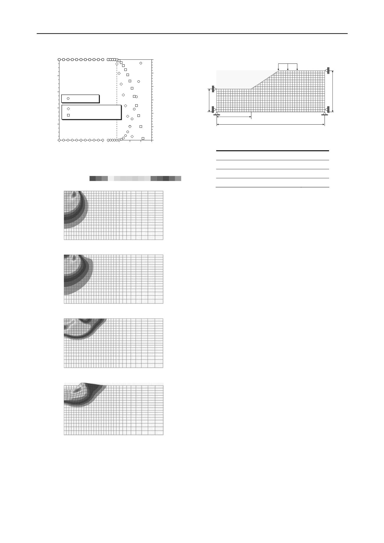
Figure 3. Relationship of the loading and the displacement acceleration,
the displacement velocity, the displacement
(a) Loading
:
84.0 kPa
(b) Loading
:
99.0 kPa
(c) Loading
:
105.0 kPa
(d) Loading
:
116.0 kP
Figure 4. The collapse mode and the equivalence strain velocity
distribution by the dynamic deformation analysis
shown to occur deformation if the loading exceeds 105.0 kPa
(Figure 3). It indicated that the proposed method can obtain
similar result against the Prandtl’s theoretical solution and the
limit bearing capacity analysis because this loading value is the
limit bearing capacity. In addition to that, we show the
equivalence strain velocity distribution and the deformation
mode against each loading at the Figure 4. It indicated that
36.0
94.0
30.0
20.0
1:1.5
0
F
Figure 5. Analysis model [Length unit : m]
Table 2. Analysis condition
Angle of shear resistance
[°]
10.0
Cohesion
c
[kPa]
50.0
Unit weight
γ
t
[kN/m
3
]
18.0
Initial loading
F
0
[
kPa
]
180.0
max
e
min
e
occur the equivalence strain velocity of the bulb form at the
initial loading. After it indicated the similar deformation mode
against the Prandtl’s theoretical collapse mode with increase of
the loading.
It indicated that the rigid plastic dynamic deformation analysis
can evaluate properly against the limit bearing capacity
problems of the horizontal ground from the above simulation
results.
4 VERIFICATION OF EFFECT BY THE LOADING
HISTORY
This chapter will verify applicability of the proposed method
against deformation behavior by the loading history such as
increase or decrease. We show the analysis model at the Figure
5. This model has inclination of slope of 1
:
1.5. The loading
applied to top of slope as the loading velocity of 10.0 kPa/sec
(time interval
t of 0.1 sec/step). The boundary condition of
displacement gave the restraint condition of the model bottom
and the horizontal restraint condition of the model side. The
parameter assumed the cohesive soil (the Table 2).
4.1
The limit bearing capacity analysis
We show result of the limit bearing capacity analysis at the
Figure 6. This Figure shows the equivalence strain velocity
distribution and the collapse mode. Here, this collapse mode is
expressed from displacement which multiplied displacement
velocity to any time. It obtained the collapse mode which shows
the slip line (the large shear zone of the equivalence strain
velocity) of the circular arc form toward the toe of slope from
the top of slope as result of the limit bearing capacity analysis.
And it obtained 195.94 kPa as the limit bearing capacity.
4.2
The bearing capacity deformation analysis
Next, we show result of the deformation analysis considering
the loading history against the bearing capacity problem of
slope at the Figure 5. We carried out three cases of the case [1]
constant increase, the case [2] keep after constant increase, the
case [3] decrease after constant increase, as the analysis cases.
In addition, we carried out comparison of calculation based on
the infinitesimal deformation theory or the finite deformation
theory because it verify effect of the geometry form. Both
theories obtained 196 kPa as the same limit bearing capacity
against the limit bearing capacity analysis's result because the
displacement increased after the loading exceeds the loading
196 kPa. We show the collapse mode based on the finite
deformation theory in the case [1] at the Figure 7. This collapse
mode is expressed from the displacement which it is obtained
from the deformation analysis. This collapse mode obtained


