700
Proceedings of the 18
th
International Conference on Soil Mechanics and Geotechnical Engineering, Paris 2013
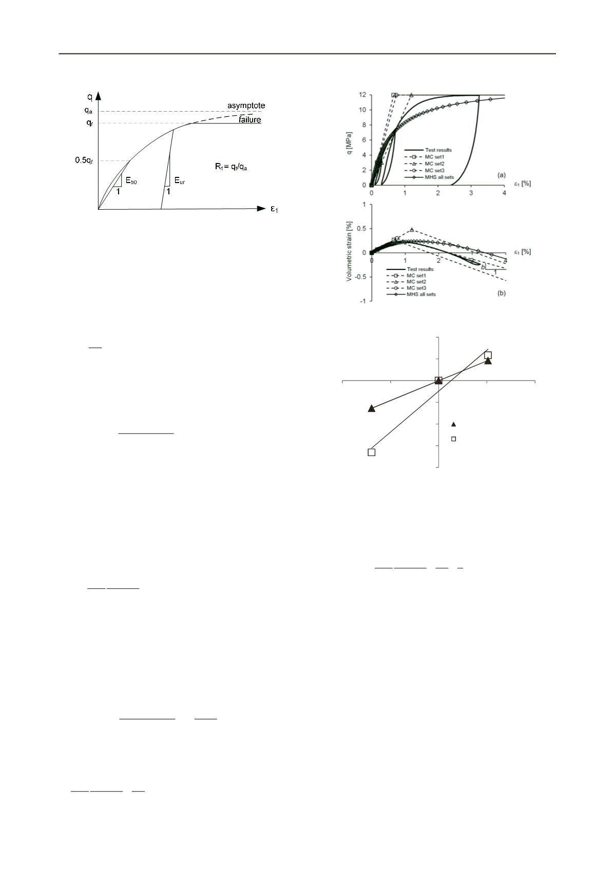
Figure 1. Hyperbolic stress-strain relationship in a CD triaxial test.
The MHS model is formulated within the framework of elasto-
plasticity; the axial strain
1
is divided into an elastic part and a
plastic part:
1 1
1
e
p
(1)
The elastic part of the axial strain depends linearly on the
deviatoric stress
q
(Fig. 1).:
1
e
ur
q
E
(2)
where
E
ur
denotes the elastic unloading-reloading modulus. The
latter depends in general on the minimum principal stress
3
according to the following power law:
3
,
cot
cot
m
f
f
ur
ur ref
ref
f
f
c
E E
p c
,
(3)
where
E
ur,ref
,
c
f
and
φ
f
denote the modulus at a reference
pressure
p
ref
, the final cohesion and the final friction angle
,
respectively. The two shear strength parameters are identical
with the cohesion and the friction angle of the standard MC
model.
The MHS model adopts the basic idea of the HS model,
which is to formulate the plastic part of the axial strain in such a
way, that the overall response during primary loading in drained
triaxial tests fulfill
s Duncan and Chang’s (1970) hyperbolic
relationship:
1
50
1
2 1 /
a
q
E q q
for
q
q
f
,
(4)
where
q
a
and
q
f
denote the asymptotic deviatoric stress and the
deviatoric stress at failure, respectively (Fig. 1). The latter is
usually taken equal to a fraction of the asymptotic stress (i.e.,
q
f
= R
f
q
a
, where
R
f
is a constant).
E
50
is the secant stiffness in
primary loading at
q
= 0.5
q
f
and depends on the minimum
principal stress
3
via the same power law as the unloading-
reloading modulus does:
3
50,
50
50,
,
cot
cot
m
f
f
ref
ref
ur
ref
f
f
ur ref
c
E
E E
E
p c
E
.
(5)
From Eqs (1), (2) and (4) we obtain the following relationship
between the deviatoric stress and the plastic axial strain:
1
50
1
0
2 1 /
p
a
ur
q
q
E q q E
.
(6)
Figure 2. (a) Deviatoric stress and, (b), volumetric strain as a function of
axial strain under a radial stress of 5 MPa (parameters: Table 1)
y = 0.9104x - 0.0041
R² = 1
y = 1.884x - 0.2424
R² = 0.9671
-2
-1.5
-1
-0.5
0
0.5
1
-1
-0.5
0
0.5
1
LN(
E
/
E
ref
)
LN(
3
*
/
p
ref
*
)
un-/reloading stiffness
secant stiffness
Figure 3. Relationship between
E/E
ref
and
3
*
/p
ref
*
in a log-log scale
Since the material is continuously yielding during primary
loading, the left-hand-side of Eq. (6) represents the yield
function:
50
1
2
( ,
)
2 1 /
3
ps
ps
s
s
a
ur
q
q
f
E q q E
.
(7)
This formulation contains as hardening parameter the plastic
shear strain
ps
s
instead of the plastic axial strain
1
p
. This
substitution is possible provided that the plastic volume changes
are relatively small (
1
3
1
1
1.5 0.5 1.5
ps
p
p
p
p
p
s
vol
).
During hardening, the mobilized shear strength parameters
increase from zero to their final values. The yield function (Eq.
7) can be written in terms of the mobilized friction angle
m
. In
order to reduce mathematical
formalism, we apply Caquot’s
(1934) transformation to the normal stresses and formulate the
yield condition and plastic potential in terms of the transformed
average and deviatoric stresses, which reads as follows:
*
*
*
1
3
)
(
2 / 3
cot
f
f
p
p c
(8)
*
*
*
1
3
q
q
.
(9)
During yielding the stresses fulfill the Mohr-Coulomb criterion
with the mobilized friction angle
m
(Eq. 10). At failure,
q
reaches
q
f
and
m
reaches
f
in Eq. (10).


