696
Proceedings of the 18
th
International Conference on Soil Mechanics and Geotechnical Engineering, Paris 2013
optimal preconditioners for such problems. Comparing Eqs. (1)
and (2):
1
2
1
2
with
.
T
T
T
T
P L B
T
K B
A
L G B
K
P L
B C
L
B B C
G
)
1
The to
(3
where
P
is the stiffness matrix corresponding to stiff materials,
G
is the (soft) soil stiffness matrix,
L
is the stiff material-soil
connection matrix, and
B
= [
B
1
,
B
2
]
T
. The proposed block
diagonal preconditioners have the following form:
(4)
)
(5
where,
1
1
2
2
is
an
approximation to the Schur compelement matrix and α is a non-
zero parameter, which is set to -4 based on an eigenvalue
theorem developed in (Phoon et al. 2002). Whether a material is
considered stiff so that the use of above preconditioners can be
advantageous is largely problem dependent. Our numerical
experiences suggest that the material 1 would be considered
stiffer than material 2 if the ratio of Young’s modulus of
material 1 (E
1
) to material 2 (E
2
) is greater than 300-400 for the
use of above preconditioners.
1
ˆ
( )
( )
T
T
S C B diag P B B diag G B
In general, the linear system is more prone to numerical
instability (even with direct solvers) if this ratio grows very
large. However, the theoretical block diagonal preconditioner
has turned this curse into an advantage (see the theorem in
Chaudhary et al. 2012), which is the basis of these inexact block
diagonal preconditioners. Thus, an even better performance can
be achieved if the problem involves several orders of difference
in stiffness properties. This is because the sensitivity of stiffness
contrast of materials is effectively minimized when the
submatrix
P
is solved directly (such as Cholesky factorization)
in
M
1
and
M
2
. The only limitation of the above preconditioners
is that the size of submatrix
P
should be such that its direct
factorization is not very expensive to compute with the
available random access memory (RAM) of the computer.
However, the memory demands of these preconditioners are
still much more affordable than applying an incomplete LU
factorization preconditioner to the entire
A
or even entire
K
,
because the size of
P
is usually much smaller than that of
A
(or
K
) for most of the geotechnical problems. The preconditioner
M
2
has an edge (up to about 2 times faster) over
M
1
due to the
modified symmetric successive over-relaxation approximation
(Chen et al. 2006) of lower-right 2×2 submatrix of
A
. This is
also helpful in minimizing the effect of contrasts in hydraulic
conductivity of the materials. However,
M
1
is easier to be
implemented and parallelized than
M
2
. Both of these
preconditioners have been implemented in GeoFEA.
2 CASE STUDY – BASEMENT EXCAVATION
2.1
Site Condition
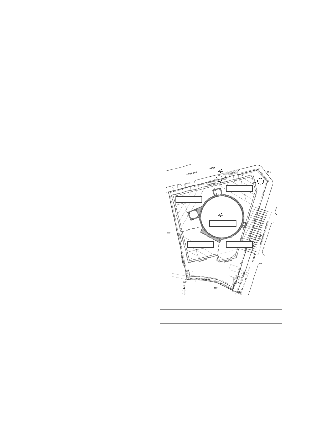
Figure 1 shows the plan view of the excavation site. The 36
storey condominium housing development project has 2 levels
of basement excavation for carparks at Ardmore Park,
Singapore. As shown in Figure 1, there are three types of
retaining systems used in this project: (1) Circular sheet pile
cofferdam with concrete ring waling in WS-A, (2) Corner strut
system in WS-B, WS-D and WS-E, and (3) Ground anchors in
WS-C and WS-D. The ground surface was sloping downwards
from North (RL 117.5m) to South (RL 112.5m). The depth of
excavation varies due to sloping ground and was about 14m for
the central cofferdam area (WS-A), and about 7.7m for outside
it.
p 1.8m to 5.5m of soil is fill material with average
SPT N-values estimated to be 3. This is underlain by residual
soil derived from Bukit Timah Granite Formation. This residual
zone is classified into GVI-1 and GVI-2 with a thickness
ranging from 7.1 to 11.8m and 4.4 to 8.9m respectively. The
residual zone is followed by zones of completely weathered
Bukit Timah Granite Formation, GV-1 and GV-2. GV-1 ranges
from homogeneous to non-homogeneous subsurface material
with thickness varying from 3.1 to 10.0m. The SPT N-values
lies between 24 and 51. The thickness of GV-2 zone is from 5.7
to 7.7m with SPT N-values lying between 53 and 94. The soil
underneath consists highly weathered Bukit Timah Granite
Formation GIV with SPT N-values well above
100blows/300mm. Most of the excavations are carried out in
residual soil derived from Bukit Timah Granite Formation.
Table 1 shows the soil properties used in the analysis.
1
0
0
0
( )
0
ˆ
0 0
(
P
M diag G
diag S
)
2
2
2
0
with
0 MSSOR( )
T
G B
P
M
H
B C
H
A
Figure 1. Plan view of the project site with strutting system
Table 1. Idealized soil profile used in the analysis.
Sub-
layer
Fill
GVI-1 GVI-2 GV-1 GV-2
GIV
Hard
Stratum
Depth
(m)
0-
14.3
1.8-
20.6
9.7-
27.9
12.8-
35.6
18.9-
37.7
26.1-
43.9
25.5-
41.2
SPT
value
0-12
6-24
11-47 24-62 50-100 >100
>100
E,
kN/m
2
9,000 15,000 38,000 80,000 155,000 650,000 950,000
c',
kN/m
2
1
5
7
5
20
150
200
',
degree
26
27
28
34
34
36
36
'
0.3
0.3
0.3
0.3
0.3
0.3
0.3
k,
m/s
5×10
-8
2×10
-7
1×10
-7
1×10
-7
1×10
-7
1×10
-6
1×10
-6
OCR
1.5
1.2
1.2
1.1
1.1
1.1
1.1
A
1
2
WS-D
WS-E
WS-A
WS-B
WS-C


