697
Technical Committee 103 /
Comité technique 103
2.2
Finite Element Analysis
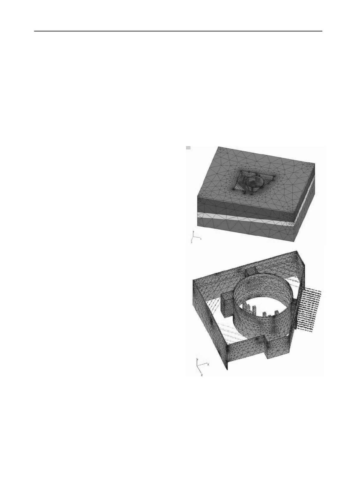
The finite element analysis was conducted using GeoFEA
version 9.0 (2012). The finite element mesh of the model is as
shown in Figure 2. The geometry and ground profile were
closely tried to replicate the real situation. The dimension of the
model is 176m long by 141m width. The total number of
elements used is 198,127 inclusive of 53,673 elements for
structural elements. The structural elements are sheet pile,
struts, walers, piles, etc. in this analysis, as shown in Figure 2b.
This generated a total degrees-of-freedom (DOFs) of 855,645.
Note that in the excavation analysis, the total DOFs changes in
each stage due to excavation of soil (removal of elements) and
installation of struts (inclusion of elements). Hence, the stiff
DOFs (related to stiff materials) as well as total DOFs vary for
different construction stages. The stiff DOFs range from
227,028 to 248,034 in different stages which are in the range of
30 to 40% of the total DOFs in respective stages. The element
types used in the analysis are as follows:
a) Steel struts and walers were modeled using 3-noded linear
elastic beam elements. A preload of 100kN was applied at
each strut. This was achieved in GeoFEA by applying
100kN load at each connection point of struts with walers
before installing the struts.
b) The sheet piles were modeled using 10-noded tetrahedron
elements. The section modulus of the 0.3m wall is taken to
that of equivalent to the section modulus (EI) of the FSP
IV sheet pile, which has been used in the site.
c) All soil types were modeled using 10-noded tetrahedron
elements. All soil types were modeled using Mohr-
Coulomb models with associated flow rule.
The side boundaries are restrained laterally and the bottom
boundary is fixed in all directions. The water table is set at RL
112.5m, lowest ground surface level in the model, so that no
area is inundated. The sheet pile was assumed to be wished-in-
place.
To model the whole excavation process, 41 increment blocks
(or stages) were necessary besides the initial step (0) to compute
the initial stresses. The excavation was carried out parts-by-
parts as marked in Figure 1. The excavation was started from
WS-A up to RL 101.5m, and followed to WS-D, WS-C, WS-B
and WS-E up to 108m, respectively. The construction sequence
consisted of alternate layers of excavation and installation of
struts. Four layers of circular ring beam were installed within
the circular pit as strutting system for the excavation from RL
115.5m to RL 101.5m. After excavating to the desired level, the
pile cap and tower footing were constructed, 4
th
ring at RL
104m was removed, and backfilled up to RL 107.1m. Similarly,
the excavation at WS-D was carried out to RL 108m with 2
levels of strut at corners and 2 levels of soil anchors inclined at
an angle of 10
downward into the ground near WS-C. WS-C
has only one level of strut at RL 110m as the excavation depth
is shallower that other zones due to sloping ground. Note that,
in actual construction, the soil anchors were replaced by raker
system. Areas WS-B and WS-E both have two levels of corner
struts at RL 113m and RL 110m, and RL 115m and RL 111m,
respectively. Total pore pressures boundary conditions were set
to zero on each exposed faces after excavation to represent a
dried excavation pit. A surcharge of 2kPa was applied to each
slope cuts as to represent the 10mm thick lean concrete.
All the stages were modeled with 5 load increments to
account for nonlinear soil behavior except for the final
excavation stage of WS-E, which was modeled with 20 load
increments. This was decided to reduce the out-of-balance loads
redistribution by the Newton-Raphson method resulting from
equilibrating the external and internal forces. This gives a total
of 221 load increments including in situ stress computation.
As linear elastic model was used for structural elements and
Mohr-Coulomb model with associated flow rule was used for
all soil types, the coefficient matrix
A
(Eq. 1) is symmetric
indefinite. Hence, the symmetric quasi-minimal residual
(SQMR) solver (Freund and Nachtigal 1994) was used in
conjunction with
M
1
and
M
2
preconditioners for the solution.
The solution with
M
2
-SQMR was completed in 48 hours and 11
minutes. Thus, the average solution time for each load
increment was 13.1 minutes only. However, the average time
for
M
1
-SQMR was about 20 minutes for each load increment.
This is considerably faster, given the size and complexity of the
problem. The solution was carried out on DELL XPS 8300
Intel® Core™ i7-2600 CPU @ 3.40GHz with 16GB RAM.
Note that, there is no memory issue for the same sized problem
on a PC with 8GB RAM as well. This shows that the large-scale
simulations involving materials of strongly varying material
properties are feasible for routine geotechnical analyses using
above solvers in GeoFEA.
(a)
(b)
Figure 2. Finite element mesh: (a) Overall geometry, and (b) Structural
elements and strutting system
2.3
Two-Dimensional Idealization
Various types of idealizations are frequently made in the finite
element analysis of many geotechnical problems in order to
simplify the analysis. However, geometric idealization is often
situational and less amenable to generalization compared to
other idealizations such as numerical or material (Lee, 2005).
The studied problem was also analyzed with two-dimensional
plane strain and axisymmetric analyses along a section A-A, as
shown in Figure 1, to compare the outputs.


