463
Technical Committee 101 - Session II /
Comité technique 101 - Session II
ε
c
=ψ(D
r
)0.0226e
2.04D
lnN
(3)
Secondly, assume that static and dynamic stress level is
equivalent. Static stress parameters are as follows:
D
r
=q/q
f
, q=σ
1
-σ
3
, σ
1
—axial load
,
q
f
---failure strength.
Thirdly, assume that time and cyclic number is equivalent.
N=t. N—cyclic number, t—creep time (h).
Finally, dynamic parameters are instead of static parameters.
ψ(D
r
) is introduced. Then the creep strain formula can be
obtained:
ε
c
=ψ(Dr)0.0226e
2.04D
lnt
(4)
. D=q/σ
3
ψ(D
r
)is a function of stress level. By analyzing the test data,
the formula under different condition can be fitted as follows:
Drained condition: ψ(Dr) = 1.52e
0.67Dr
(5)
Undrained condition: ψ(Dr) = 0.07e
3.61Dr
(6)
The strain under different stress level and drainage condition
can be calculated by Eq. 4, Eq. 5 and Eq. 6. The calculation and
test results can be seen in Figure 6 and Figure 7.
Figure5. Creep Test and Calculation Results under Drained Condition
0.0
0.5
1.0
1.5
2.0
2.5
3.0
3.5
4.0
0
500
1000
1500
2000
Axial permanent strain ε
(
%
)
Cyclic Number
(
N
)
orTime
(
hour
)
42.5kPa test results
42.5kPa calculation results
40.5kPa test results
40.5kPa calculation results
31.0kPa test results
31.0kPa calculation results
14.8kPa test results
14.8kPa calculation results
Figure 6. Creep Test and Calculation Results under Undrained
Condition
The creep time under drained condition is longer than
undrained. The developing trend and magnitude of strain which
is calculated are in accordance with test results and the long-
term creep deformation is predicted. The calculation results of
31.0kPa and 40.5kPa deviate from test results under undrained
condition. The reason may be that the function
ψ
(D
r
) is an
approximate expression which comes from limited test data.
There might be other factor or correlation. It is the next work to
solve.
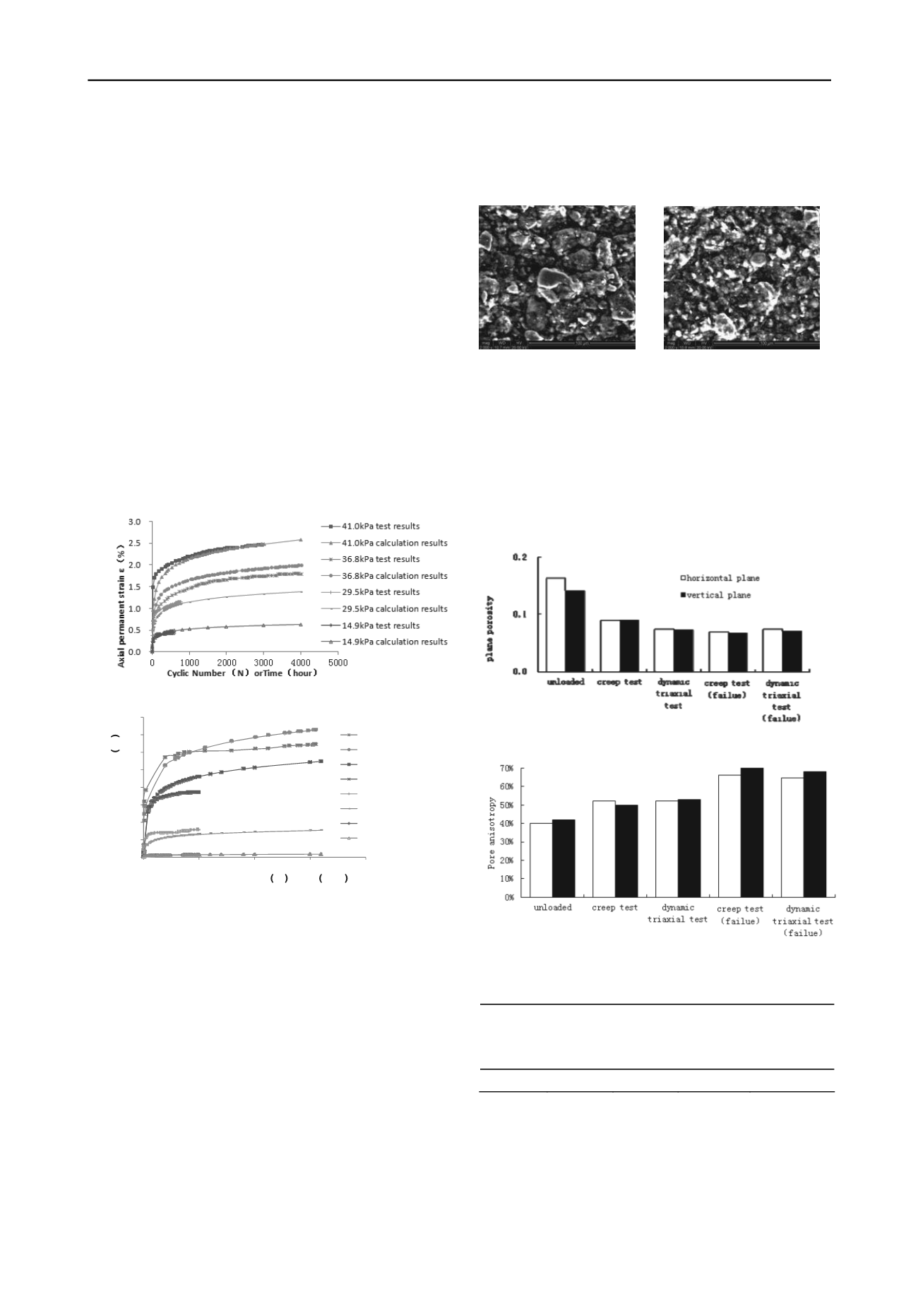
3 MICROSTRUCTURE ANALYSIS
In order to explicit the microstructure change after the creep and
dynamic triaxial test, the SEM test was carried out in low
vacuum mode. The SEM test instrument is Quanta400 scanning
electron microscope. The soil sample was cut to a cube of
1.5cm
×
1.5cm
×
1.5cm by wire saw. Both vertical and horizontal
plane was test. The porosity parameters of soil including plane
porosity, anisotropy and directional probability entropy were
counted to analyse the microstructure change. The image of soil
was magnified 2000 times, and the microstructure photographs
before and after loading were shown as Figure 8 and Figure 9.
Figure 7. Unloaded soil SEM Figure 8. Soil SEM photograph
photograph after creep test
Figure 10, Figure 11 and Table 5 shows the microstructure
parameter of different test. Both the vertical and horizontal
plane porosity decreased after creep and dynamic triaxial test.
The increasing anisotropy of porosity means that the porosity’s
shape trends to oval. The porosity directional probability
entropy increases after creep and dynamic triaxial test. When
the soil samples failure, the porosity directional probability
entropy of creep soil sample is similar with dynamic triaxial test.
Fig 9. soil sample plane porosity of different test
Fig 10. Porosity anisotropy of different test
Table 4. directional probability entropy of Porosity
unloaded
Creep
test
dynamic
triaxial
test
Creep test
(failure)
dynamic
triaxial test
(failure)
0.982
0.91
0.86
0.81
0.823
4 CONCLUSIONS
1. The creep deformation and permanent deformation of
dynamic triaxial test are nonlinear. The deformation in
macrostructure is a pattern of appearance of microstructure
change.


