371
Technical Committee 101 - Session II /
Comité technique 101 - Session II
Proceedings of the 18
th
International Conference on Soil Mechanics and Geotechnical Engineering, Paris 2013
The specimens with the 10% and 14% initial water
contents, and a high soil structure, exhibit relatively rigid elastic
behavior at the early stage of loading and show brittle behavior
at the following stage. Plastic behavior can be observed from
the early stage for the specimens with the 0% and 3% initial
water contents without a high soil structure.
4 . SIMULATION BY SYS CAM-CLAY MODEL
It can be assumed that the difference in the test results due to
the initial water contents is caused by the soil structures that
form in the specimens during the specimen preparation. In this
study, a numerical simulation is performed to confirm this
assumption using the superloading and subloading Cam-clay
model named SYS Cam-clay model (Asaoka et al. 2002), which
can describe the effects of the soil structure. The SYS Cam-clay
model incorporates the concepts of the soil stucture, over-
consolidation and anisotropy into the modified Cam-clay model.
In e SYS Cam-clay model, the soil structure is assumed to
deteriorate with an increasing the plastic shear strain.
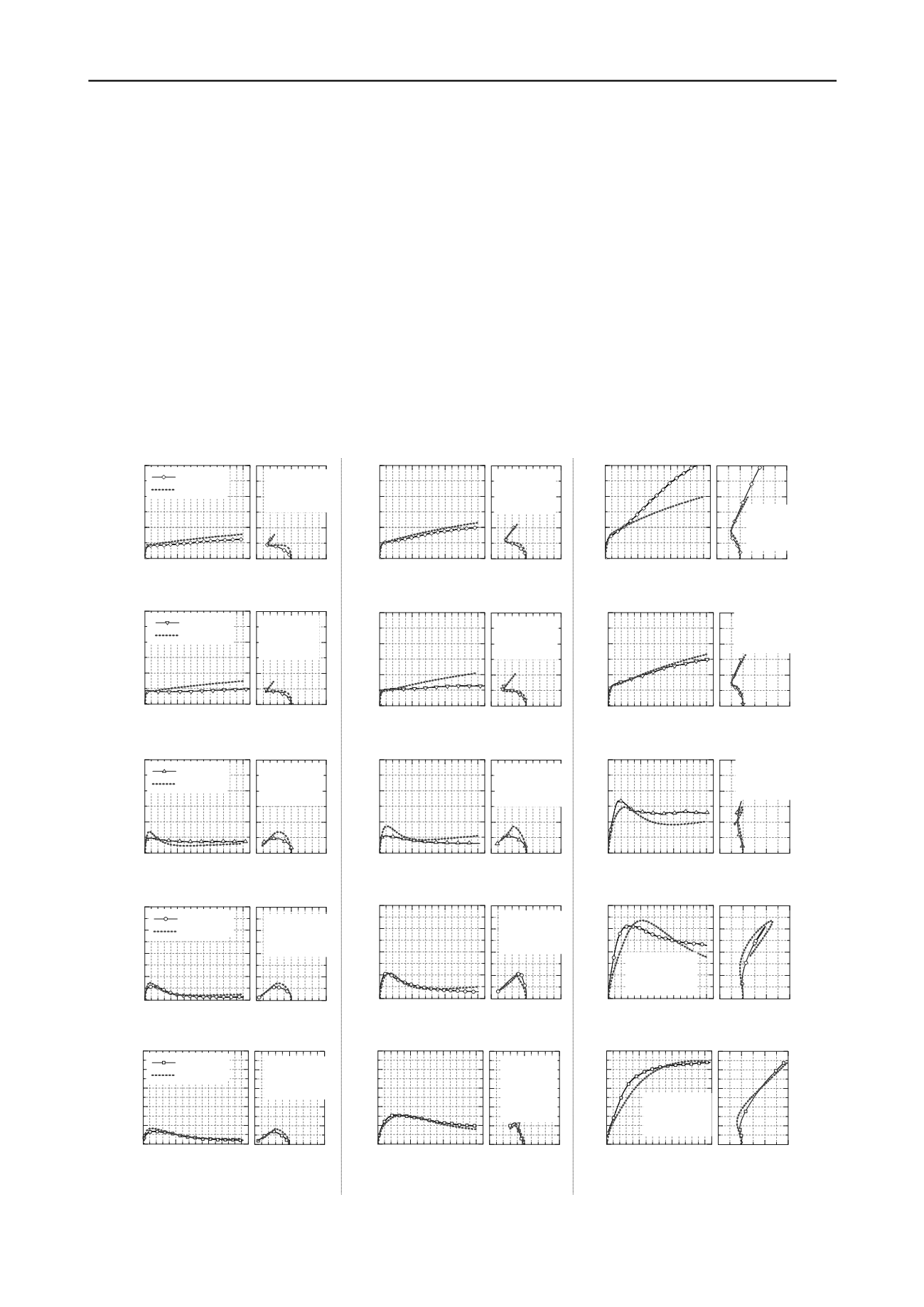
Figure 4 illustrates the simulation results with the values
of the parameters for the soil structure used in each case. In this
analysis, the initial values for the degree of soil structure 1/
R
0
*
,
initial overconsolidation ratio 1/
R
0
and soil structure
degradation parameter
a
are defined as variables in order to
explain the various complicated types of behavior of the
structured soil. From the triaxial test results, it is assumed in this
study that higher soil structures are generated in the specimens
with higher initial water contents. Therefore, a higher the initial
value for the degree of soil structure 1/
R
0
*
is set in the case of a
higher initial water content. Furthermore, a smaller
a
value is
adopted in that case, since the high soil structure may not be
easily deteriorated due to shearing. Thus, parameter
a
expresses
the rate of degradation of the soil structure and the larger value
for
a
describes faster degradation of the soil structure. The other
parameters used in this study, i.e., elasto-plastic parameters,
evolution law parameters and initial conditions, are in common
and are listed in Table 1. Since 1/
R
0
*
and 1/
R
0
are dependent on
each other, when 1/
R
0
*
is set first, 1/
R
0
is automatically
determined from the values of an initial specific volume
v
0
and
Initial water content 0%
Initial water content 5%
Initial water content 0%
Initial water content 0%
Initial water content 3%
Initial water content 3%
Initial water content 3%
Initial water content 5%
Initial water content 5%
Initial water content 10%
Initial water content 10%
Initial water content 10%
Initial water content 14%
Initial water content 14%
Initial water content 14%
(a)
D
= 80%
(b)
D
= 85%
(c)
D
= 90%
0
5 10 15
0
100
200
300
triaxial test
simulation
q
(kPa)
s
(%)
0 100 200
p'
(kPa)
1/
R
0
*
=2.6
1/
R
0
=6.5
a =
18
Triaxial test
Simulation
Triaxial test
Simulation
Triaxial test
Simulation
Triaxial test
Simulation
0
5 10 15
0
100
200
300
q
(kPa)
s
(%)
0 100 200
p'
(kPa)
1/
R
0
*
=2.0
1/
R
0
=10.0
a =
16
0
5 10 15
0
100
200
300
q
(kPa)
s
(%)
0 100 200 300
p'
(kPa)
1/
R
0
*
=1.1
1/
R
0
=11.9
a =
10
0
5 10 15
0
100
200
300
t i
l test
sim tion
q
(kPa)
s
(%)
0 100 200
p'
(kPa)
1/
R
0
*
=2.8
1/
R
0
=6.8
a =
17
0
5 10 15
0
100
200
300
q
(kPa)
s
(%)
0 100 200
p'
(kPa)
1/
R
0
*
=2.4
1/
R
0
=10.9
a =
15
0
5 10 15
0
100
200
300
q
(kPa)
s
(%)
0 100 200 300
p'
(kPa)
1/
R
0
*
=1.7
1/
R
0
=14.9
a =
10
0
5 10 15
0
100
200
300
triaxial test
s lation
q
(kPa)
s
(%)
0 100 200
p'
(kPa)
1/
R
0
*
=14.0
1/
R
0
=15.7
a =
2.8
0
5 10 15
0
100
200
300
q
(kPa)
s
(%)
0 100 200
p'
(kPa)
1/
R
0
*
=13.0
1/
R
0
=32.0
a =
2.7
0
5 10 15
0
100
200
300
q
(kPa)
s
(%)
0 100 200 300
p'
(kPa)
1/
R
0
*
=12.0
1/
R
0
=62.9
a =
2.0
0
5 10 15
0
100
200
300
400
t iaxial test
s m lation
q
(kPa)
s
(%)
0 100 200
p'
(kPa)
1/
R
0
*
=24.0
1/
R
0
=22.1
a =
2.7
0
5 10 15
0
100
200
300
400
q
(kPa)
s
(%)
0 100 200
p'
(kPa)
1/
R
0
*
=23.0
1/
R
0
=51.1
a =
2.6
0
5 10 15
0
100
200
300
400
q
(kPa)
s
(%)
0 100 200 300
p'
(kPa)
1/
R
0
*
=22.0
1/
R
0
=108.5
a =
1.0
0
5 10 15
0
100
200
300
400
500
triaxial test
simulation
q
(kPa)
s
(%)
0 100 200
p'
(kPa)
1/
R
0
*
=18.0
1/
R
0
=18.4
a =
1.5
0
5 10 15
0
100
200
300
400
500
q
(kPa)
s
(%)
0 100 200
p'
(kPa)
1/
R
0
*
=18.
0
1/
R
0
=41.7
a =
1.0
0
5 10 15
0
100
200
300
400
500
p'
(kPa)
q
(kPa)
s
(%)
0 100 200 300
1/
R
0
*
=12.0
1/
R
0
=62.9
a =
0.3
Triaxial test
S lation
Triaxial test
Si ulation
S
Triaxial test
Si ulation
r ax a e
Figure 4. Numerically simulated stress- strain relations and effective stress paths with various initial water contents.


