205
Technical Committee 101 - Session I /
Comité technique 101 - Session I
Proceedings of the 18
th
International Conference on Soil Mechanics and Geotechnical Engineering, Paris 2013
higher than K
0
determined from oedometric yield point and the
empirical correlation of Mayne and Kulhawy (1982) K
0
=1.2.
4
NUMERICAL ANALYSIS OF MARCHETTI
DILATOMETER
An attempt was made to explain this discrepancy by numerical
modelling of the flat dilatometer penetration into the soil. For
the numerical analysis the hypoplastic model (Mašín, 2005) was
used in combination with the intergranular strain concept
(Niemunis and Herle, 1997). The model predicts nonlinear
stiffness depending on the strain level. The input value of K
0
of
1.2 was considered. Both the calibration and the parameters for
the hypoplastic model were taken from Svoboda et al. (2010)
and Mašín (2012). The parameters are summarised in Table 1.
Table 1. Parameters of the hypoplastic model
φ
c
λ*
κ*
N
r
22°
0.128
0.015
1.51
0.45
m
R
m
T
R
β
r
χ
16,75
8.375
1.e-4
0.2
0.8
The numerical analysis was carried out using Plaxis 2D
finite element code. The modelling sequence involved three
phases:
1. Generation of the initial stress condition with K
0
= 1.2,
2. Excavation of the 5.5 metres thick layer in order to reach
the measured pore water pressure of -32 kPa at the depth of 11.7
metres. Consolidation time was varied using the consolidation
analysis until the measured excess pore water pressure was
obtained.
3. The installation of the dilatometer was simulated in a
simplified manner using two approaches. In the first one,
displacement was prescribed at the left boundary of the model,
as depicted in Fig. 2. The second analysis involved prescribed
load. The dilatometer was 200 millimetres high and 14
millimetres wide (7 mm horizontal displacement was
considered in the model thanks to its symmetry) and it was
installed in the depth of 11.6 – 11.8 metres. In the analyses,
load/displacement was evaluated in the centre of the
dilatometer. These phases employed a plastic undrained
analysis.
Figure 2. Distribution of horizontal displacements calculated by the
hypoplastic simulation of Marchetti (1980) dilatometer.
The calculated coefficient K
D
was 4.51 for the load
controlled analysis and 4.06 for the displacement controlled
analysis, which leads to K
0
equal 1.07 and 1.00 respectively.
This preliminary analysis thus indicated slight underprediction
of K
0
using Marchetti (1980) empirical equation. Limitations of
the model need, however, be considered. In particular the
simplified geometry and limitations of the adopted constitutive
model, which does not allow for an explicit consideration of
inherent stiffness anisotropy. To overcome this limitation, a new
anisotropic version of the hypoplastic model is currently being
developed.
5
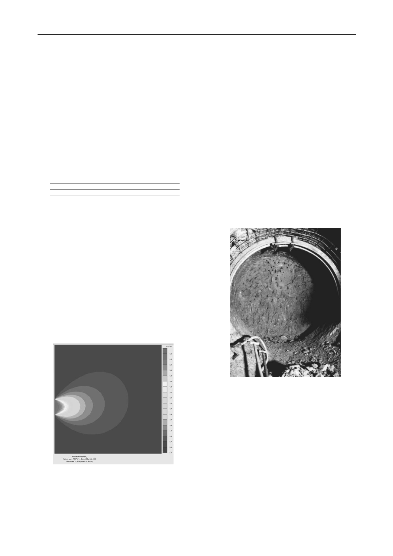
BACKANALYSIS OF CIRCULAR ADIT
In the second numerical study presented, the K
0
coefficient is
evaluated by means of backanalysis of convergence
measurements within a circular exploratory adit. The adit was
excavated as part of a geotechnical site investigation preceeding
the excavation of Královo Pole Tunnels in Brno (see Svoboda et
al., 2010).
The adit was located 26 m below the ground level, and its
diameter was 1,9 m. Its geometry is shown in Fig. 3. The adit
was protected by a steel net and rolled steel arches. These were
installed for safety reasons only, and the support was never in
full contact with the cavity wall. The monitored convergence of
the cavity is thus assumed to be representative of the
displacement of an unsupported massif. Its convergence was
monitored by means of push-rod dilatometer in four different
directions (vertical, horizontal and two sections inclined at 45
degrees).
Figure 3. Circular adit used in backanalyses of the earth pressure
coefficient at rest K
0
(Pavlík et al., 2004).
The adit has been simulated in 2D and 3D using finite
element method. The model properties were taken over from
Svoboda et al. (2010). Hypoplastic model parameters are in
Tab. 1. In the analyses, it was assumed that the massif
properties were known. The initial value of K
0
was varied by a
trial-and-error procedure until the model correctly reproduced
the measured ratio of horizontal and vertical convergence of the
adit. The analyses were performed under undrained conditions.
The analyses were performed using the softwares PLAXIS
2D and PLAXIS 3D. The 2D analyses adopted the load
reduction method (see Svoboda and Mašín, 2011). In these
analyses, the load reduction factor was varied to achieve the
monitored displacement magnitude, and the coefficient K
0
was
adjusted to reproduce the ratio of displacements in horizontal
and vertical directions.
Geometry assumed in the 3D analyses is in Fig. 4. No effort
was made to vary model properties to reach the exact monitored
displacement magnitude. As in 2D analyses, K
0
was


