142
Proceedings of the 18
th
International Conference on Soil Mechanics and Geotechnical Engineering, Paris 2013
16
Capillary
Barrier
60
mm
30
mm
Monolithic
Cover
60
mm
Resistive
Cover
15 mm
45
mm
Gravel
(
k
= 0.1 m/s)
Uncompacted Soil
(
k
= 1.4 x 10
-6
m/s)
Compacted Soil
(
k
= 6.9 x 10
-8
m/s)
(a)
10
-8
10
-7
10
-6
10
-5
10
-4
10
-3
10
-2
10
-1
0 100 200 300 400
(b)
Capillary Barrier
Monolithic Cover
Resistive Cover
Normalized Oxygen Diffusion
Coefficient,
D
N
Time (d)
Figure 20. Gas-phase oxygen diffusion through three types of soil
covers: (a) cross sections of cover types; (b) normalized oxygen
diffusion coefficients at 0.6-m depths within the soil covers (data
from Stormont et al. 1996; modified after Shackelford 1997).
5 DIFFUSION IN REMEDIATION APPLICATIONS
In terms of remediation, failure of the pump-and-treat
technology to achieve clean-up goals has been attributed,
in part, to the process of "reverse matrix" or "back"
diffusion resulting in the slow and continuous release of
contaminants from the intact clay and rock matrix into the
surrounding, more permeable media, such as fractures or
aquifer materials (e.g., Mackay and Cherry 1989, Mott
1992, Feenstra et al. 1996, Shackelford and Jefferis 2000,
Chapman and Parker 2005, Seyedabbasi et al. 2012).
Diffusion also has long been recognized as the transport
process that controls the potential leaching of contaminants
from stabilized or solidified hazardous waste, typically by
the addition of pozzolanic materials such as cement, lime,
and fly ash (e.g., Nathwani and Phillips 1980). Finally,
diffusion may be a significant transport process with
respect to controlling the rate of delivery of chemical
oxidants (e.g., potassium permanganate, KMnO
4
) injected
into contaminated low-permeability media through
hydraulic fractures for
in situ
treatment of chlorinated
solvents (Siegrist et al. 1999, Struse et al. 2002).
5.1
Reverse Matrix or Back Diffusion
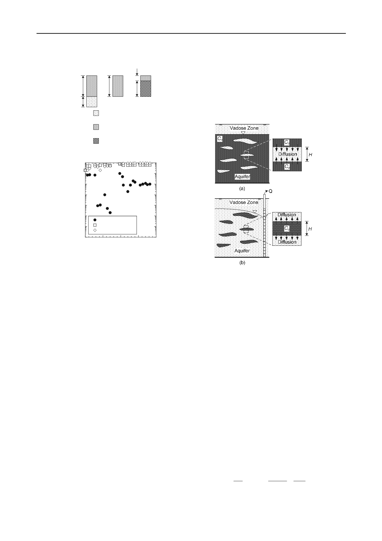
As an example of reverse matrix or back diffusion,
consider the scenario illustrated conceptually in Fig. 21a,
where initial contamination of the aquifer results in a
difference in concentration between the contaminated
aquifer and the clay lens resulting in diffusion of
contaminants into the porous matrix of the clay lens. After
pumping commences, the higher permeability portion of
the heterogeneous aquifer is flushed of contamination
relatively quickly, resulting in a reversal of the
concentration gradient and an outward diffusive flux of the
contaminant (Fig. 21b). This outward or reverse matrix
(back) diffusion process results in a slow release of
residual contamination back into the aquifer that can lead
to failure of the pump-and-treat remediation technology to
achieve regulatory levels within a short time frame, leading
to extensive pumping and excessive costs (e.g., Feenstra et
al. 1996).
Figure 21. Matrix diffusion and reverse matrix diffusion: (a)
diffusion into clay lens before pump-and-treat remediation; (b)
reverse matrix or back diffusion out of contaminated clay lens
during pump-and-treat. (modified after Shackelford and Lee
2005).
The effect of matrix diffusion on pump-and-treat
remediation can be analyzed via superposition of an
analytical solution based on the analogy between
consolidation and diffusion and the principle of
superposition (Shackelford and Lee 2005). For example,
consider the case where the aquifer is initially
contaminated with trichloroethylene (TCE) at a
concentration,
C
o
, of 1000 ppm, such that TCE diffuses
into a 1-m-thick (=
H
) clay lens for a period of time.
However, before the clay lens becomes completely
contaminated, pump-and-treat remediation is undertaken to
clean up the aquifer. As a result, the initial TCE
concentration profile within the 1-m-thick (=
H
) clay lens
is sinusoidal as a result of incomplete matrix diffusion of
TCE into the clay lens prior to pumping, with a maximum
TCE concentration of 1000 ppm at the aquifer-clay
interface and a minimum contaminant concentration of 300
ppm at the center of the clay lens. This initial distribution
of contaminant within the clay lens is represented in Fig.
22a in terms of the relative concentration,
C
(
Z
,
T
*
)/
C
o
, of
TCE as a function of the dimensionless depth,
Z
,
corresponding to a value of the dimensionless diffusive
time factor,
T
*
, of zero (
T
*
= 0), where (Shackelford and
Lee 2005):
*
*
2
2
;
a
d
d d
d
D t
z
D t
Z
T
H
R H H
(8)
and
H
d
is the maximum diffusive distance (=
H
/2 or 0.5 m
in this example). The definition for the dimensionless


