2871
Technical Committee 212 /
Comité technique 212
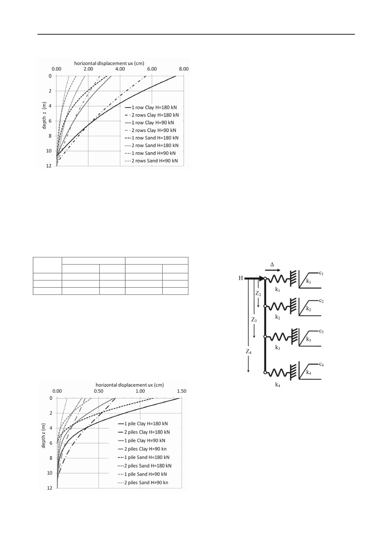
Figure 1. Lateral deflections for 1- and 2-row pile groups
.
Table 2 lists the calculated lateral deflections consistent with the
loads and soils shown in Figure 3. While the elastic/plastic
behavior allowed for nonlinear load-displacement curves,
deflections from these two programs were consistently lower
than Plaxis-2D. There is also reason to believe that the two
subgrade reaction programs may better represent single piles (as
in 3D, discussed later) than as a 2D “pile wall” as represented in
Figure 1.
Table 2. Summary of reaction coefficients and displacements
Axis
Geo 4
Spring
Mode
k (MN/m/m) ux (cm) Ch (MN/m
3
) ux (cm)
Elastic
15-45
0.66
19-56
0.88
Elas/Plas
15-45
1.35
19-56
1.70
Elas/Plas
30-90
1.09
19-56
0.65
4 COMPARING 3-D ANALYSES
3-D methods highlight the same behavior but to different
degrees. Using similar soil properties, one may compare the
benefit of a two-pile system. The 3D model also made use of
interface elements and a thin pile element placed within the
solid element pile in order to determine shear and bending
moments (MIDAS 2009). This time, the benefit is more
pronounced, due to the more efficient process of spreading
reaction loads throughout the soil in three dimensions.
Figure 2. Displacement profiles for 1, 2 piles; Sand, Clay; 90,180 kN.
Displacement magnitude is much less for all combinations of
load and soil. Surface displacements are smaller than those in
Figure 3 by a factor of about 5-8x. This time the number of piles
resisting movement is more influential in reducing displacement
than the soil modulus. This is evidenced by the fact that the
displacement profiles are grouped by number of piles and load
magnitude (1 pile Sand H=180 is most near to 1 pile Clay
H=180, etc.) The single piles also show a very pronounced
slope at the surface which will again translate to rigid body
rotation of the bridge pylons.
5 COMBINING ANALYSES
Presently the research group is adapting an optimization method
to translate pile head displacement and rotations computed from
2D and 3D finite element analyses to a small number of elasto-
plastic subgrade springs for use in structural or geotechnical
design software (such as GEO and AXIS). The method assumes
the pile has identical structural properties as the original (more
sophisticated) analysis software. Four to six lateral springs are
placed on the pile at various depths. One spring is always placed
at the surface, another at the pile tip. The remaining springs will
be placed in optimal positions to produce similar responses at
the top of the pile.
The procedure seeks to optimize three quantities for each
spring: elastic constant, k; plastic limit, c; and depth were the
spring is attached to the pile, z. The pile structural element is
modeled as a series of beam elements with nodes located at the
pile tip, point of application of the middle springs, and the pile
top. For a four spring model, the pile will consist of four nodes
and three elements (Figure 5).
.
Figure 3. Four element pile with elasto-plastic springs.
The optimization process varies the eight spring parameters
and two depths (the other two are the fixed length of the pile
and zero) to minimize the least squares error between the
deflection, Δ, computed above and the displacement generated
from the finite element model for the same load, H. When the
sum of least-squares error is minimized, the problem is solved.
This is the same process one uses for fitting trend lines to data.
The program is written in Visual Basic for Applications (VBA)
and runs within an Excel spreadsheet. Computing deflections
for the various loads is done with a small, nonlinear matrix
structural analysis program that is called as an Excel function
and returns the computed deflection value to the spreadsheet.
The optimization makes use of the Solver add-in found in
Excel. The parameters that are varied in the solver are those
discussed above, the target value to minimize is the sum of the
squared errors. Sample output for the optimization process is
shown in Figure 6.


