2246
Proceedings of the 18
th
International Conference on Soil Mechanics and Geotechnical Engineering, Paris 2013
size. f(x)
i
is the objective function (here FOS of i
th
individual).
The technique is known as windowing as it eliminates the worst
individual (FOS)-the probability comes to zero, and stimulates
the better ones.
Within the random generated set of population (n) of design
multivariable (N-dimensions or feature vectors),
f
(x
i
, y
i
, z
i
,…w
i
)
within wide deterministic search boundaries for each variable,
and subsequent objective function evaluations, the minimum is
located. With a view to exp oit the search space neighbourhood
the N-multivariable set
l
min
min
min
min
i
i
i
i
,...w z, y, x
f
creating
this minimum is perturbed by a factor (
k) sequentially in both
directions (positive as well as negative directions)
Δk
w,...
Δk
z,k
min
min
i
i
Δ y,Δk
x
min
min
i
i
f
to
create
1 22
! i Ni!
N!
N
2 C 2
Ni
1i
Ni
1i
i
N
offspring
{Where, N!=N.(N-1).(N-2)…….3.2.1} in the neighbourhood of
the local minimum in an attempt to generate some superior
offspring. Hence, for a three variable function (like slope-
stability problem)
f{
(x
i
),(y
i
),(z
i
)}, a population (of n individuals)
are randomly generated and their local minimum
min
min
min
i
i
i
z,
y,
x
f
located for the first generation.
Thereafter, this local minimum is perturbed initially in the
positive direction and function evaluatio are made at
ns
Δk y,Δk
z,Δk y,
Δk z, y,
z , y,Δk
min
min
min
min
min
min
min
min
min
min
min
i
i
i
i
i
i
i
;Δk z,
z, y,Δk xf ;Δk
z,Δk y,Δk xf ;
; z,Δk y, xf ;
min
min
min
min
min
min
min
min
min
min
i
i
i
i
i
i
i
i
i
i
;Δk
;
xf
xf
xf
xf
i
i
i
i
and finally in the negative direction, by changing the sign of
k
in above expressions. Hence, apart from objective function
evaluations of all n number of population individuals in each
generation, the algorithm requires further function evaluations
at 2(2
N
-1) points around the local minimum of each generation.
Now as fresh generations are produced, often different selection
pressures of reproduction are needed at successive generations.
Hence, the choice of a value of the sequential perturbing factor
(
k) becomes of paramount importance, in a sense that if it is
too large it will be adequate in the first phase of the search but
not in the final phase and vice versa if it is too small. Further,
this
k is likely to be different for different design variables
commensurate with their individual feasible search intervals. As
such, the situation calls for some sort of normalization of
k in
initial phase for application in various problem domains, and
further it should possess the flexibility of shrinking itself
automatically in successive generations according some decay
rule in compliance with the selection pressure criteria. In this
study, this perturbing parameter is defined as
k=
.(x
i
U
-x
i
L
).
i
,
where,
is a problem specific constant; to be fixed after some
initial trials. x
i
U
and x
i
L
are the upper and lower bounds of a
design variable and
i
[=G
i
(1-r)
(Gi-1)
] is the size reduction
parameter, where, G
i
is the generation number and ‘r’ a constant
less than unity. As the number of design variables (N-
dimensions) increases, more trials are needed for fixing the
value
of
.
The
‘fittest’
perturbed
offspring
min
i
p
,...w
min
min
min
i
p
i
p
i
z , y ,
p
xf
of the i
th
generation decides
a new contracted search interval for the consecutive generation,
wherein the value each design variable corresponding to the
fittest perturbed offspring is assigned the central value of the
interval. The two new extreme bounds of the fresh search
interval is the product of the positive and negative value of this
central value and the size reduction parameter,
i
. Thus, if the
local minimum objective function of the previous generation be
min
min
min
min
1-i
p
1-i
p
1-i
p
1-i
p
w,...
z,
y,
x
f
, the current (that
is,
i
th
)
search
interval
becomes,
i
p
1) (i
p
1) (i
1G
i
p
1) (i
i
p
1) (i
p
1) (i
1G
i
p
1) (i
min
min
i
min
min
min
i
min
1G w,...
z r1G z
1G y ,
x r1G x
p
1) (i
1G
p
1) (i
1G
min
i
min
i
w r
,
y r
.
A new population of random variables (of size n) is again
generated from
scratch
within the new reduced stochastic
search interval and again objective function evaluations are
made for each set of new random variables so generated. The
generated set replaces the initial one and the loop is continued
to produce fresh generations of refined offsprings till the
outcome converges to the global optima.
2.1 APMA efficacy checked with benchmark test functions
With a view to examine the performance of the algorithm,
APMA is initially applied to some benchmark unconstrained
global optimization test functions like Goldstein-Price’s
function, Hartman’s function, Beale’s function, Perm’s
function, Booth’s function, Bohachecsky’s function (A. Hedar),
Six hump camel’s back function and Xin-She-Yang’s function
(X.-S. Yang, 2010) and promising results were obtained.
APMA successfully captured all the four optima of the
multimodal Himmelblau function (Deb K., 2000):
f(x
1
,x
2
)=(x
1
2
+x
2
-11)
2
+(x
1
+x
2
2
-7)
2
,
[
the optima being
(-2.805,
3.131); (-3.779, -3.283); (3.584, -1.848); (3,2)
] in each and
every simulation run while finally converging to the global
minimum at
(3,2)
[
The simulation runs has been done with
=80-90% & r=0.10
]. The method may be regarded as a basic
thrust of ‘Artificial Intelligence’, that is to get the computer to
perform tasks fast and automatically. The method is
independent of the initial vector and as no specific search
direction is used in this method, this random search method is
expected to work efficiently in many classes of problems.
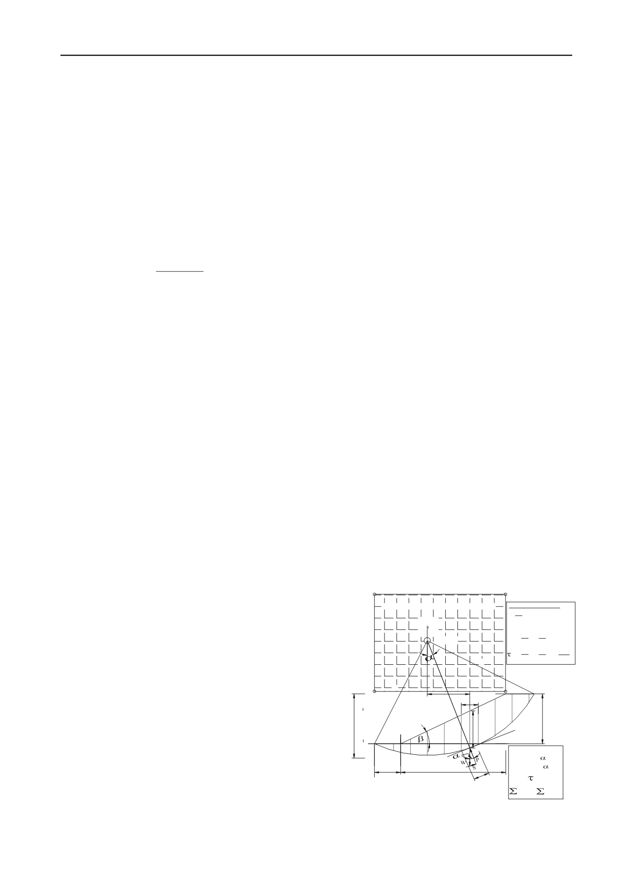
3 THE PROBLEM DEFINITION
A problem cited by Spencer (1967) is chosen for analysis. The
problem parameters, soil-data and search boundaries are
depicted in Fig.1. In the search process, the three independent
design variables are the abscissa (CX) and ordinate (CY) of the
circle centre and the depth factor (N
d
) of the circular failure
surface. The base width (B) and height (H) of slope are assumed
as 60 meters and 30 meters respectively.
CX, CY
R
R
B=60
H=30
N H
(0,0)
0.25B=15
d
(B, 1.05H)
(B, 3H)
(-0.25B, 3H)
(-0.25B, 1.05H)
u
c = 0.02
= 40 deg.
SUB-SOIL DATA
r = = = 0.50
H
/
/
O
Center
of
circle
INITIAL FEASIBLE SEARCH SPACE
0.80 < Initial N < 1.25
d
b
h i
i
i
i
i
W =b h
i i i
= tan (H/B)
-1
ub
W
u
h
l
b = l cos
S = l
i
i i
i
i
i
i
i
x
W x = S R
i i
i
x =R sin
i
i
i
= + ( - u)
c
F
P
l
tan
F
/
/
Fig.1. Initial variable bounds of the tri-variable & soil data used in
search for critical circle-
The Slope-Stability problem definition
.
The radius R=f{CX, CY, N
d
H}. Based on a few trials, the
feasible bounds of the design variables, has been identified as: -


