1732
Proceedings of the 18
th
International Conference on Soil Mechanics and Geotechnical Engineering, Paris 2013
0,
βy
,
0,
(1)
A parameter
α
stands for a size of a loosened zone with respect
to the width D. Another parameter
β
is a magnitude of a
velocity which can be negligible due to the first order of
homogenuity in upper bound calculations.
2.2 Calculation of dissipation rate
Internal dissipation rate per unit volume can be expressed as in
Eq. (2) in terms of mean effective stress
p’
and deviatoric stress
q
.
w
σ
∙ ε
p′ ∙ ε
q ∙ ε
(2)
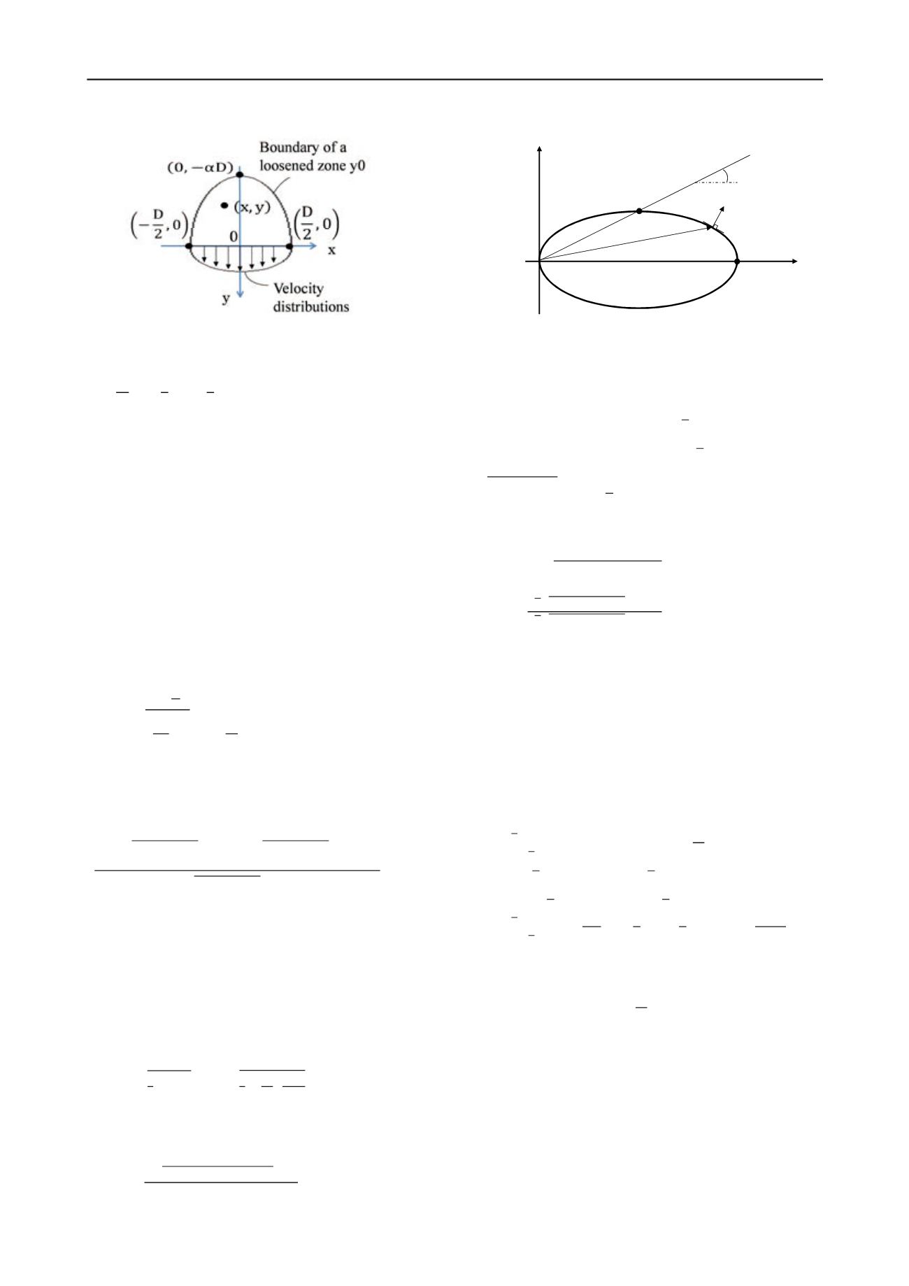
For a case of modified Cam-clay model (Figure 3), internal
dissipation rate should be derived from its yielding function (Eq.
3) and associated flow rule (Eq. 4) :
f p
∙
p
=0
(3)
ε
λ ∙
ε
λ ∙
(4)
Concrete form of internal dissipation rate for modified Cam-
clay soil is as follows,
w
ε
ε
ε
ε
ε
ε
ε
p
(5)
where
p
and
M
stand for a maximum consolidation stress and a
gradient of a critical state line which is can be uniquely
determined by tri-axial compression tests.
Volumetric plastic strain rates
ε
and deviatoric plastic
strain rates
ε
for assumed failure modes are as follows,
ε
ε
ε
ε
β
(6)
ε
e
e
β
∙
(7)
By substituting Eqs. (6) and (7) into Eq. (5), internal dissipation
rate per unit volume is shown as
w
∙ p
(8)
Total internal dissipation rate is then calculated by integrating
Eq. (8) over a volume,
W
w
x ∙ dv 1 ∙ w
dx dy
p
βD
55296α
M
18432
√34
9192
4
9
(9a)
Where
A
and
k
are as follows,
A 48
4
9 2304
96
216
(9b)
k log
√
√
(9c)
In this formulation, a closed-form solution of
W
can be
obtained.
2.3 Calculation of external plastic work rate
External plastic work rate consists of two terms;
W
done by
self-weight of a soil in a loosened zone and
W
due to
uniform upward pressure q.
W
γ u
dv
γ ∙ βy y
dv
=
γ ∙ βy y
dy dx
γα
βD
(10)
W
q ∙ u
dx
=
q ∙ βy
dx
=
q ∙
x
x
dx
(11)
External plastic work rate
W
is then calculated as follows,
W
W
W
αβD
4γ αD 10q
(12)
2.4 Evaluation of uniform pressure q to stabilize a trap
door
According to the upper bound theorem, a following inequality
holds if a structure is stable for the assumed failure mechanism:
W
W
(13)
Therefore, by equilibrating internal dissipation rate and external
plastic work rate in eq. (13) and arranging them with respect to
a uniform upward pressure q, a following equation can be
derived,
Figure 2. Assumed failure mode and velocity distributions
Figure 3. Modified Cam-clay model and associated flow rule
0
M
(p
y
’,0)
q, ε
d p
ε
ij p
ε
v p
,
ε
d p
σ
ij
p′, ε
v p


