1252
Proceedings of the 18
th
International Conference on Soil Mechanics and Geotechnical Engineering, Paris 2013
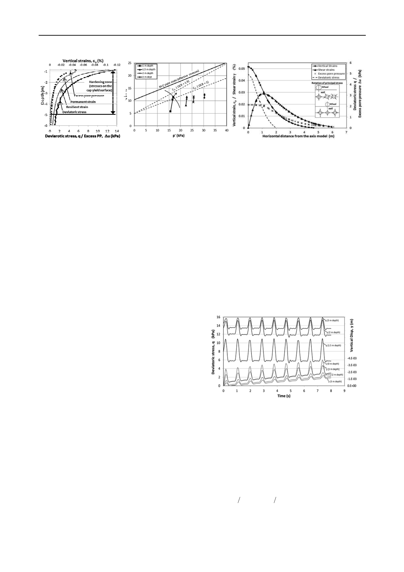
(a)
(b)
(c)
Figure 4. Subgrade response under static loading; (a) deviator stress, permanent and resilient strains, and excess pore pressure; (b) stress state at
different depths and failure criteria under drained and undrained conditions;(c) horizontal distribution of stresses and strains at 1.5 m depth.
The influence of axle load below pavement surface reaches 6
m depth, although the most of strains take place in the upper
layers of subgrade.
It is also noted that within upper 5 m the stresses reaches cap
yield surface, leading to an isotropic hardening of soil. Besides,
Figure 4b shows the stress states at different depths, where can
be seen that the current effective stress state remains far of
Mohr Coulomb failure condition, although it is near the
undrained failure e.g. according to the empirical equation S
u
=
0.35·
v
’·OCR
m
proposed by Ladd (1991), with OCR = 1 and m
= 0.85. The ratio between current deviator stress and deviator
stress at failure R=q/q
f
could be used to express the extent to
which permanent deformation might develops; usually it is
assumed that permanent deformation will start to rise for R >
0.70 – 0.75 (Korkiala-Tanttu 2008). In any case, isotropic
compression produces plastic volume strains once the excess
pore pressures are completely dissipated.
The horizontal distribution of shear and vertical strains at 1.5
m depth are shown in Figure 4c; it can be seen that in the
vertical axis, there is no shear strains and the vertical strain
reaches its maximum value, which indicates a purely triaxial
compression state just below the load. On the other hand, the
largest shear strain is located at a horizontal distance of 1.10 m
from the load, where soil is under a general stress regime with
shear and axial stresses. In reality, when cyclic load of moving
wheel over the pavement surface is applied, these two stress
state are successively changed. Also it is noted that at 1.5 m
depth the maximum deviator stress reaches values near 6 kPa,
and spreads horizontally up to 2 m from the load axis. Whereas
the influence of excess pore pressure spreads horizontally until
4.5 m, approximately.
3.4.2 Subgrade response under cyclic loading
The effect of one cyclic loading stage composed by 10 load
repetitions is shown in Figure 5; the deviator stress, as well as
recoverable and permanent displacement at different depths are
also depicted in Figure 5. In Figure 6a are shown the curves of
shear moduli degradation G
S
/G
0
and G
t
/G
0
determined by the
Equation (2) as a function of strain level and the parameters G
0
and
0.7
outlined in the table 1. Also in Figure 6a are shown the
results of finite element modelling for the maximum shear
strains produced after each iterative calculus under cyclic
loading, for a reference depth of 1.5 m. The interception of
these maximum shear strains with the curves G
S
/G
0
and G
t
/G
0
gives the proportion at which soil modulus is changed.
In a next step, stiffness are reduced due to number of load
repetitions by means of Equation 1, considering a parameter t =
0.045 (Dobry and Vucetic 1987).
It was observed that maximum shear strain obtained in the
first 10 load repetitions (
= 2.9·10
-4
) is larger than the reference
shear strains
0.7
(
1.75·10
-4
), which coincides with the proportion
of permanent deformation at this loading stage. After 20 load
repetitions the shear strain was lower than the
0.7
, and after the
subsequent load repetitions the strains were reduced more
slowly until reach values leading to ratios G
S
/G
0
= 0.82 and
G
t
/G
0
= 0.67. The OCR was gradually increased in between
each iterative calculation up to a maximum value of 1.50. In the
Table 3 are shown the results of final subgrade soil stiffness at a
reference depth of 1.5 m.
The damping ratio obtained from the adopted procedure is
verified according to the Equations (3) to (5), taking the
maximum shear strain after each iteration, in order to reproduce
a representative hysteresis loop. Thus, in total 10 damping ratios
have been estimated. In Figure 6b are shown the results of
damping ratio compared to the analytical results for hysteretic
damping considering variation of initial shear modulus G
0
from
values of 2G
ur
to 6G
ur
, and variation of
0.7
from 1·10
-4
to 2·10
-4
.
It is observed that results obtained from finite element
modelling fit well with hysteretic damping related to
0.7
=
1.75·10
-4
. In the two first iterations was obtained damping ratios
close to 0.1, which were reduced gradually until the final
iterations reached values close 0.045. This tendency agrees with
the typical reduction in the amount of permanent deformation
with the load repetitions, due to the reduction in the amount of
dissipated energy.
Figure 5. Subgrade response under cyclic loading.
3.4.3 Subgrade performance in the long term
In order to estimate the long term behavior of the soft
subgrade analyzed, one could adopt an empirical power
equation for calculating the cumulative plastic strain. Chai and
Miura (2000) proposed an enhanced formula of a former
empirical model proposed by Li and Selig (1996) for estimation
of cumulative plastic strains with the number of repeated load
applications. This new model is defined in the Equation (6),
which has demonstrated that its prediction agrees with actual
measurements taken from low height embankments on soft soil.
b n
f
is
m
f d
p
N q q1
q q a ε
(6)
Where
p
= cumulative plastic strain (%); q
is
= initial static
deviator stress; q
d
= dynamic load induced deviator stress;


