1251
Technical Committee 202 /
Comité technique 202
stress state after load repetitions, overconsolidation ratio OCR
of natural soft soil is systematically recalculated due to the
modification of the stress history. In total 10 iterations of cyclic
loading have been adopted with 10 load repetition each one, so
that the analysis reaches 100 load applications.
The decrease of clay stiffness due to increase of the load
repetitions is well known issue. To take into account this effect
Idriss et al. (1978) proposed that the decrease in modulus could
be accounted for by a degradation index
according to (1).
= (E
S
)
N
/ (E
S
)
1
= N
-t
(1)
Where: (E
S
)
N
is the secant young’s modulus for Nth cycle;
(E
S
)
1
is the secant young’s modulus for the first cycle; and t is a
degradation parameter, which represent the slope of the curve
log E
S
– logN.
On the other hand, in order to take into account the influence
of the typical small strains produced below the pavement
structures, it was assumed the soil stiffness degradation due to
strain level. Hardin and Drnevich (1972) proposed a simple
hyperbolic law to describe how the shear modulus of soil decays
with the increase of shear strains. Afterward, Santos and Gomes
Correia (2001) modified this relationship to determine de
variation of secant shear modulus G
S
as a function of the initial
(and maximum) shear modulus at small strains G
0
, and of the
shear strain
0.7
related to the 70% of the maximum shear
modulus 0.7G
0
as a threshold. Equation 2 describes this relation
in the domain of a certain range of shear strain, commonly
within values from 1·10
-6
to 1·10
-2
. The tangent shear modulus
G
t
can be determined taking the derivative of G
S
.
7.0
0
S
0.385
1
G
G
;
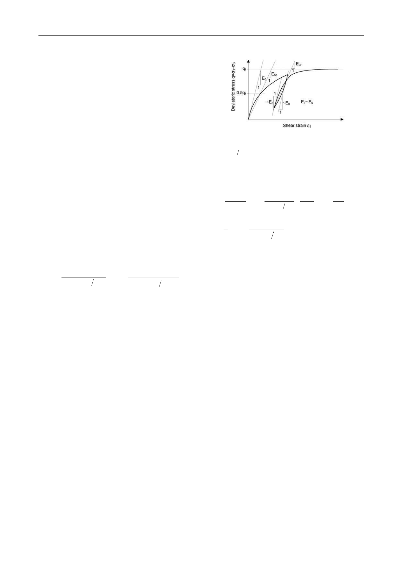
Figure 3. Hyperbolic stress-strain relation and moduli E
0
, E
50
and E
ur
adopted in the HS-small model.
S
D
Eπ4 Eξ
(3)
Where E
D
is the dissipated energy in a load cycle comprised
from the minimum to maximum shear strain (Equation 4), while
E
S
is the energy stored at maximum shear strain
c
(Equation 5).
0.7
c
0.7
c
0.7
c
c
0 0.7
D
γ
aγ
1 ln
a
2γ
aγ γ1
γ
2γ
a
G 4γ
E
(4)
7.0
2
2
0
2
S
22
2
1 E
c
c
cS
a
G
G
(5)
Where a= 0.385
2
7.0
0
t
0.385
1
G
G
(2)
This approach is based on the research carried out by
Vucetic and Dobry (1991) and Ishihara (1996), which
demonstrated that beyond a volumetric threshold strain
v
the
soil starts to change irreversibly. At this strain level, in drained
conditions permanent volume change will take place, whereas
in undrained conditions pore water pressure will build up
(Santos and Gomes Correia 2001). Furthermore, it is well
known that the degradation of G/G
0
with shear strains depends
on many factors e.g. plasticity index, stress history, effective
confine pressure, frequency and number of load cycle, etc.
Indeed, with the purpose of consider the influence of the most
importance factors on the degradation of shear moduli, Santos
and Gomes Correia (2001) used the average value of
v
related
to the stiffness degradation curves (G/G
0
= f(
)) presented by
Vucetic and Dobry (1991), in order to define a unique curve of
G/G
0
as a function of normalized strain
/
v
. In this way they
concluded that when the ratio
/
v
= 1 the best fit tends to
correspond to a ratio G/G
0
= 0.7.
This approach aids to develop the small-strain stiffness
model (HSsmall) proposed by Benz (2006) that is already
included in the latest version of Plaxis code. Unlike the standard
Hardening Soil Model (Schanz et al. 1999) where a linear stress
strain relationship controlled by the stiffness E
ur
is assumed
during unloading-reloading process, the HS-small model takes
into account hysteresis loops during loading and unloading
cycles with moduli variation among initial E
0
, secant E
50
and
unloading-reloading E
ur
stiffness (Figure 3). In fact, such model
also presents a typical hysteretic damping when the soil is under
cyclic loading due to energy dissipation caused by the strains;
Brinkgreve et al (2007) proposed an analytical formulation to
estimate the local hysteretic damping ratio according to
Equation 3:
Once assumed the calculation procedure described above,
the hysteretic damping ratio according to Equation 3 is
estimated from the strain updating after each iterative
calculation (10 iterations each consisting of ten load
repetitions), considering the calibration of soil stiffness due to
strain level (
), current stress state (OCR) and number of load
repetitions (N). Moreover, viscous damping effects may be
added by means of the rayleigh damping features of the used
Plaxis version (v8.2). Rayleigh damping consists in a
frequency-dependent damping that is directly proportional to
the mass and the stiffness matrix through the coefficients
and
respectively (C =
·
M +
·
K). In fact, the damping process
subjected to a cyclic loading should be analyzed from the
combination of two approaches: mechanical hysteretic damping
depending on the strains level, and viscous damping depending
on the time, which has to fit well with both, natural material and
load application frequency. For this purpose the values adopted
for Rayleigh coefficients are
=
= 0.01.
As small-strain stiffness model is not included in the version
8.2 of Plaxis code used here, the analytical solution of
Brinkgreve et al (2007) is adopted to verify and compare the
damping ratios between the results from the finite element
modeling and the results from such analytical solution. Finally,
the behavior of subgrade soil is analyzed regarding the
accumulated vertical strains due to the cyclic load repetitions.
3.4 Modelling results
3.4.1 Subgrade response under static loading
The settlement after construction stage rise up to 25 mm, which
should last less than few months according to the typical
projects requirements. Nevertheless, the consolidation process
may lasts between 1.5 to 2.5 years considering a soil
permeability of 10
-8
to 10
-9
m/s. Regarding the operation stage,
the maximum value of excess pore pressure due to axle load
rises up to 5.5 kPa. The response of subgrade soil when the axle
load is applied under static conditions can be appreciated
through the values of deviator stresses as well as vertical
resilient and permanent strains depending on the depth
(Figure 4a).


