 
          1036
        
        
          Proceedings of the 18
        
        
          th
        
        
          International Conference on Soil Mechanics and Geotechnical Engineering, Paris 2013
        
        
          Table 2. Test cases and degree of compaction.
        
        
          For the compaction properties, a series of compaction test were
        
        
          conducted and maximum dry density of 1.90 t/m
        
        
          3
        
        
          and the
        
        
          optimum water content of 12.3 %  were obtained.
        
        
          First of all, the sand was prepared in the acrylic mould
        
        
          (height: 100mm, diameter: 50mm) with the conditions of the
        
        
          optimum water contents and dry density of 1.50 t/m
        
        
          3
        
        
          . Dynamic
        
        
          compaction method was used with controlling its compaction
        
        
          energy and here, as shown in Table 2, two different cases were
        
        
          examined, which are Case-1 and Case-2. Case-1 is the case of
        
        
          relatively high energy in which the height of each time of
        
        
          falling rammer is 0.20 m while Case-2 is the one for low energy
        
        
          which is 0.10m for the falling weight. The weight of falling
        
        
          rammer was 9.81 N. Figure 2 shows those two cases in which
        
        
          the level of compaction is also shown in this figure. As shown
        
        
          in this figure, the amount of work was set as equal for both
        
        
          cases in each level of compaction although the degree of the
        
        
          compaction was slightly different between two cases. Table 3
        
        
          shows the conditions of CT scanning and Figure 2 shows the
        
        
          scanning area of the specimen, which was the area from 15 mm
        
        
          high and up to 55mm from the bottom of the specimen and the
        
        
          width of scanning area was 40mm. The precise contents of X-
        
        
          ray CT can be found in the references (Otani 2003 and
        
        
          Watanabe et. al. 2012).
        
        
          3 IMAGE ANALYSIS
        
        
          The characteristic of compacted soils was discussed with the
        
        
          results of CT scanning and those are not only direct result from
        
        
          image visualization but also more quantitative ones such as
        
        
          distribution of the voids in the soil using image data. In order to
        
        
          obtain quantitative results, image analysis plays an important
        
        
          role and especially, the determination of the threshold value
        
        
          between two materials such as soil particles and voids is most
        
        
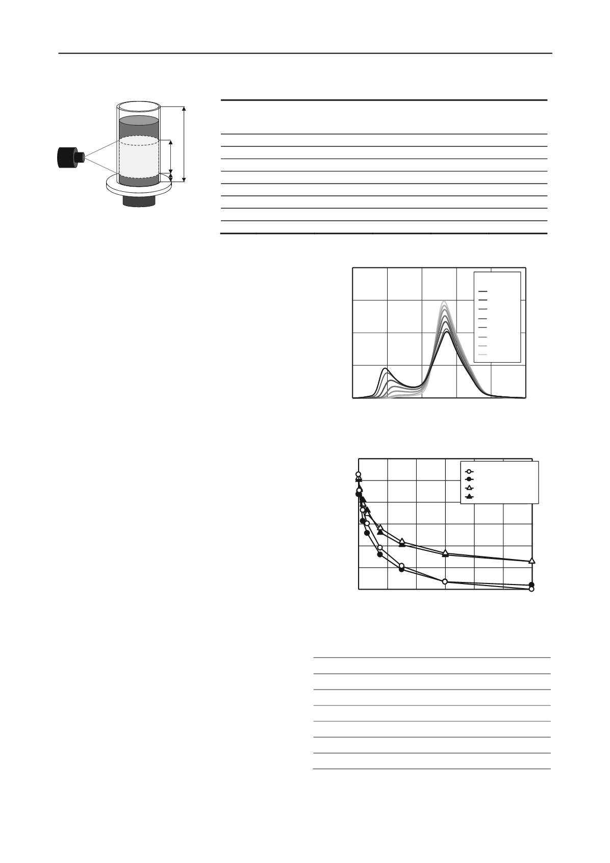
          important for this quantification. Figure 3 shows the frequency
        
        
          of so called “CT-value” in the whole specimen for Case-1. This
        
        
          “CT-value” has been known as the well correlated value with
        
        
          material density (Otani et. al. 2000). As shown in this figure,
        
        
          there are two dominant CT-values in the specimen and due to
        
        
          the level of compaction, those peaks are gradually changed. X-
        
        
          ray CT has a spatial resolution and in this case, this resolution
        
        
          was 75


          m. The sand used in this test has a fine fraction (less
        
        
          than 5


          m) of 8.2% and as a result, there is no way to
        
        
          distinguish all the sizes of the particles. However, it can be said
        
        
          from Figure 3 that the higher peak moves to the higher
        
        
          frequency and the lower peak moves to the lower frequency
        
        
          after the compaction. This means that the increase of the CT-
        
        
          value due to compaction is the cause of the fact that the small
        
        
          particles move to the voids and then those areas are shown as
        
        
          the areas of higher CT-values. In the mean time, the area of low
        
        
          density is decreased due to the decrease of the voids. In order to
        
        
          discuss more quantitative sense, the threshold value of two
        
        
          peaks shown in Figure 3 was determined. Here, EM algorithm
        
        
          (Dempster et. al. 1977) which is one of the maximum likelihood
        
        
          methods was used and this method is useful for the case of
        
        
          multiple peaks of the frequency curve. Here, the calculation
        
        
          Compaction
        
        
          Energy
        
        
          (kJ/m
        
        
          3
        
        
          )
        
        
          Case-1
        
        
          No. of
        
        
          Compaction
        
        
          Case-1
        
        
          Deg. of
        
        
          Compaction
        
        
          (%)
        
        
          Case-2
        
        
          No. of
        
        
          Compaction
        
        
          Case-2
        
        
          Deg. of
        
        
          Compaction
        
        
          (%)
        
        
          Initital
        
        
          0
        
        
          0
        
        
          79.4
        
        
          0
        
        
          78.3
        
        
          LevelA
        
        
          15
        
        
          1
        
        
          83.3
        
        
          2
        
        
          81.3
        
        
          LevelB
        
        
          75
        
        
          5
        
        
          88.2
        
        
          10
        
        
          84.7
        
        
          LevelC
        
        
          150
        
        
          10
        
        
          91.5
        
        
          20
        
        
          87.1
        
        
          LevelD
        
        
          374
        
        
          25
        
        
          97.5
        
        
          50
        
        
          90.6
        
        
          LevelE
        
        
          749
        
        
          50
        
        
          102.0
        
        
          100
        
        
          93.8
        
        
          LevelF
        
        
          1497
        
        
          100
        
        
          106.0
        
        
          200
        
        
          96.5
        
        
          LevelG
        
        
          2995
        
        
          200
        
        
          109.3
        
        
          400
        
        
          98.5
        
        
          Figure 2. Area of CT scanning.
        
        
          Scan area
        
        
          (mm)
        
        
          100
        
        
          40 15
        
        
          500 1000 1500 2000 2500 3000
        
        
          5
        
        
          10
        
        
          15
        
        
          20
        
        
          25
        
        
          30
        
        
          0
        
        
          Compaction energy (kJ/m 3 )
        
        
          Porosity (%)
        
        
          Case-1  measure
        
        
          Case-1  analysis
        
        
          Case-2  measure
        
        
          Case-2  analysis
        
        
          Voltage    (kV)
        
        
          200-230
        
        
          Current


          A)
        
        
          350
        
        
          Spatial resolution (mm)
        
        
          0.075
        
        
          Width of slice (mm)
        
        
          0.050
        
        
          Number of slices
        
        
          800
        
        
          FCD*     (mm)
        
        
          205.0
        
        
          FDD**    (mm)
        
        
          1000
        
        
          *: distance from X-ray tube to the specimen
        
        
          **: distance from the specimen to the detector
        
        
          Table 3. Condition of CT scanning.
        
        
          Figure 4. Relationship between porosity and compaction energy.
        
        
          Figure 3. Frequency of CT-value for Case-1.
        
        
          0
        
        
          50
        
        
          100
        
        
          150
        
        
          200
        
        
          8
        
        
          250
        
        
          0
        
        
          2
        
        
          4
        
        
          6
        
        
          Case-1
        
        
          initial
        
        
          Level A
        
        
          Level B
        
        
          Level C
        
        
          Level D
        
        
          Level E
        
        
          Level F
        
        
          Level G
        
        
          (
        
        
          ×
        
        
          106)
        
        
          Frequency
        
        
          CT-value