525
Technical Committee 102 /
Comité technique 102
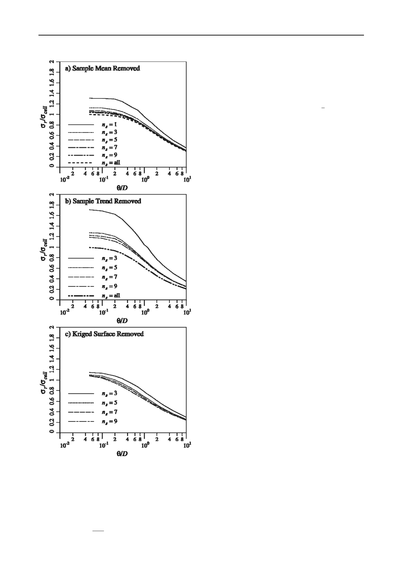
Figure 2. Standard deviation of the residual (eq. 1), normalized by the
standard deviation of
X
, versus normalized correlation length.
A possibly better measure of how well
represents the
field is obtained by considering the standard deviation of the
residual,
r
(see eq. 1), directly. This measure will include
the effects of trend removal and is illustrated in Figure 2, again
with the standard deviation of the residual,
r
ˆ
x
X
x
, divided by the
standard deviation of
,
cell
X
. In detail, the standard deviation
of the residual is estimated as the square root of the variance,
1
2
2
1
ˆ
1
n
i
i
r
i
X
n
x
x
for each realization. The value of
r
used in Figure 2 is
averaged over all realizations. As in Figure 1, the
1
s
n
case
only appears in Figure 2a, since bilinear trend and Kriging
surfaces are not well defined for only one sample point.
However, Figures 2a and b now include a limiting case where
the entire simulation has been sampled (
s
all), representing
the best site knowledge possible. This case was not included in
Figure 1 since, when all values are sampled,
n
0
r
, that is, the
average residual is zero. In Figure 1, this would have
corresponded to a horizontal line at zero standard deviation. In
Figure 2, the ‘
s
n
all’ case corresponds to the classical case
where both the estimated mean (trend) and the variance are
computed from the same set of observations. As the correlation
length decreases, these observations become increasingly
independent, and the estimated standard deviation approaches
the true standard deviation, so that
r
cell
1.
/
0
as seen in
Figures 2 a and b when
s
n
all. In Figure 2 c, the case ‘
s
n
all’ is not included in the Kriging surface case since, when the
entire field is sampled, the residual is zero with zero variability,
and so the curve corresponding to this case lies at zero.
As in Figure 1, Figure 2 also shows that the ability of
ˆ
x
to represent
X
x
improves as the correlation length
increases, for all of the trends considered. In the limit, as
/
D
, all random fields become uniform (under the
assumed finite variance correlation structure), random from
realization to realization, but constant within each realization. In
this limiting case, the sample perfectly predicts the uniform
field, and the residual becomes zero everywhere so that
0
r
.
It is apparent in Figure 2 that all curves are heading towards 0,
as
/
D
.
One of the perhaps surprising results of Figure 2 is that the
removal of a bilinear trend is not generally as good as the
removal of the constant sample mean at smaller correlation
lengths, and especially at a lower number of samples. The
reason for this becomes apparent when, for example, the case
where
3
s
n
is considered. If the correlation length is small,
then the three samples will be largely independent, and the
resulting fitted bilinear plane could (and often does) end up with
quite an unrepresentative slope, leading to a high variability in
the residual. Even when
9
s
n
the residual variability is higher
at low correlation lengths than seen using the constant sample
mean. At low correlation lengths, the Kriging surface performs
about the same as the constant sample mean.
At large correlation lengths, e.g.
/
1
D
0
, the bilinear
trend performs better than the constant sample mean for all
s
n
except
3
s
n
, where the relative standard deviation is 0.35
versus 0.32 for the constant sample mean. For higher number of
samples, the relative standard deviation using the bilinear trend
is 0.25, versus 0.31 for the constant sample mean. The Kriged
surface performs the best out of the three methods (relative
standard deviation of 0.30) when the number of samples is 3,
and about the same as the bilinear trend for higher numbers of
samples.
The last measure of the quality of the trend type used
considered in this paper is how well the estimated correlation
length agrees with the actual correlation length, Figure 3. Once
ˆ
x
has been established from the soil samples, the
correlation length is estimated here using the following steps;
1. for each direction through the soil domain,
1, 2
i
,
2. estimate the semi-variogram along all lines through the
domain in direction
i
using the entire
X
x
field,
r
3. average the semi-variograms obtained in step 2 to obtain
the final semi-variogram estimate in direction
i
,
4. fit a theoretical semi-variogram, having parameter
(correlation length), to the semi-variogram estimated in
step 3 by minimizing the sum of squared errors (i.e.
regression).
(3)


