524
Proceedings of the 18
th
International Conference on Soil Mechanics and Geotechnical Engineering, Paris 2013
Sampling at all locations is, of course, prohibitively
expensive and would also change the resulting field properties
while measuring them (see, e.g., Heisenberg, 1927). In practice,
soil properties are estimated from a relatively small number of
samples so that
will only ever approximate
in some
way (i.e., via a trend).
ˆ
x
X
x
In assessing the ability of
ˆ
x
to represent
X
x
, it will
also be useful to consider the average residual over the domain,
1
1
1
ˆ
r
r
i
n
i
D D
X d
X
D D
n
x x
x
x
i
(2)
where
D
is the edge dimension of the
D D
square domain.
The domain is broken up into
cells in the simulation,
resulting in the summation form on the right, in which is the
location of the center of the ’th cell.
n
i
x
i
ˆ
The agreement between
and
will be determined
here by considering three measures; 1) the standard deviation of
the residual field average,
x
X
x
r
(i.e., how well does the estimated
trend represent the actual field average?), 2) the standard
deviation of the residual,
r
(i.e. how much residual
uncertainty remains?), and 3) the residual correlation length (i.e.
how does the trend removal affect the perceived correlation
lengths?).
X
Five sampling schemes are considered in the paper, ranging
from a single sample taken at the field midpoint to nine samples
taken over a 3 x 3 array at the quarter points of the field. In
some cases a further ‘maximum' sampling scheme is performed,
where every point in the field is sampled, to see what the
maximum attainable uncertainty reduction is.
For each sampling scheme, three types of trend removal are
performed; a) removing the constant sample mean, b) removing
a bilinear trend surface which is fit to the sample, and c)
removing a Kriged surface fit to the sample. The residual
statistics are determined by Monte Carlo simulation, with 2000
realizations for each case, where the field is discretized into 128
x 128 cells and the random fields generated using the Local
Average Subdivision method (Fenton and Vanmarcke, 1990).
2 RESULTS
Consider first the average of the residual,
r
, given by Eq. 2. It
can be shown that the mean of
r
is zero, so that a measure of
how accurately
represents
ˆ
x
X
x
can be obtained by
looking at the standard deviation of
r
– small values of this
standard deviation imply that
ˆ
x
remains close to the field
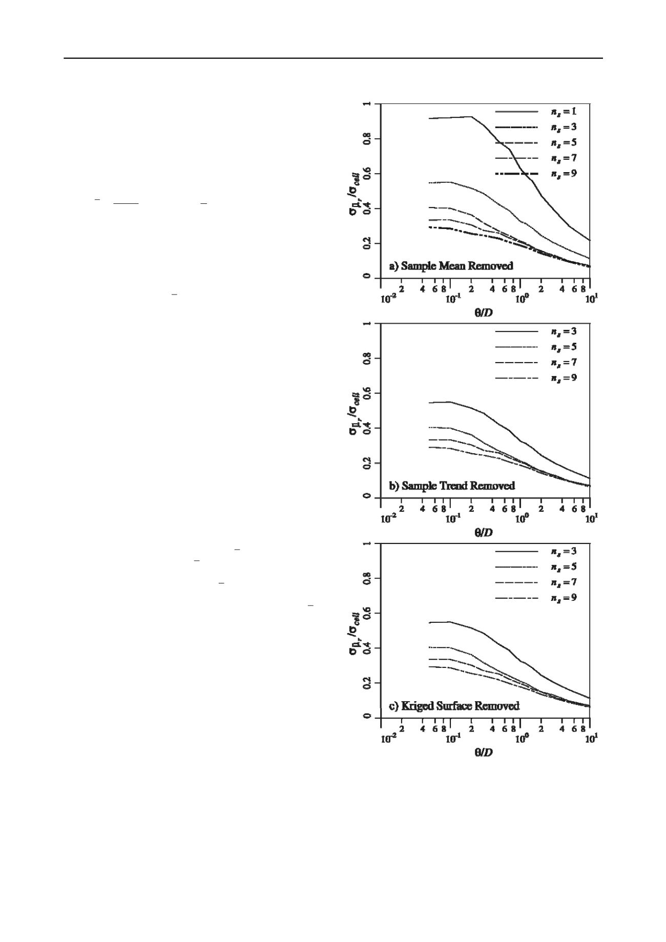
average. Figure 1 illustrates how the standard deviation of
r
,
normalized by dividing by the standard deviation of the random
field value,
, in the ’th cell (referred to as
cell
X
x
i
i
), varies
as a function of the number of samples taken from the domain,
s
n
, and the normalized correlation length,
/
D
. Note that if
only one sample is taken at the midpoint of the domain,
s
1
n
,
then a bilinear trend cannot be fit to the sample, nor is a Kriged
surface removal attempted. Thus, parts b and c in Figure 1 do
not have a curve corresponding to
s
. In all plots it is
apparent that as the number of samples increases, the accuracy
improves (in agreement with the findings of Lloret-Cabot, et al.,
2012). It can be seen, however, that for
s
to 9, there is
very little difference between the detrending methods, so far as
the field average is concerned. It is to be noted that the field
average is a constant, not a trend, so it is not expected that the
bilinear and Kriged surface trends will do any better than the
sample mean, when compared to the field average.
1
3
n
n
Figure 1. Standard deviation of the field average residual (eq. 2),
normalized by the standard deviation of
X
, versus normalized
correlation length.
In all cases in Figure 1, the agreement between
ˆ
x
and
X
x
improves as the correlation length increases. This is
because the field becomes increasingly smooth, or flat, as the
correlation length increases, so that all trends considered
become closer to the flatter
X
x
.


