257
Technical Committee 101 - Session I /
Comité technique 101 - Session I
Proceedings of the 18
th
International Conference on Soil Mechanics and Geotechnical Engineering, Paris 2013
density but also by the state variable
related to the imaginary
increase of density (bonding effect). Larger values of the state
variables
and
can be assumed to have more effects for the
degradation of
and
. Then, the evolution rules of
and
can be given in the following form, using increasing functions
G
(
) and
Q
(
) which satisfy
G
(0)=0 and
Q
(0)=0, respectively:
( )
p
d
G Q d e
(14)
Simply, the evolution rule of
is also given using
Q
(
) by
( )
p
d Q d e
(15)
The distance (
-
0
) of the two NCLs in Figure 5 is expressed as
a function of the elapsed time
t
or the rate of plastic change in
void ratio (-
e
・
)
p
, referring to the interpolated diagram in Figure
1.
0
0
0
0
( )
ln
ln
ln( )
ln( )
( )
p
p
p
p
t
e
e
e
t
e
(16)
Its increment is given by
1 ( )
p
d
dt
dt
e dt
t
t
(17)
Now, it is assumed that Equations (16) and (17) hold not only
for normally consolidated soils but also for over consolidated
soils and naturally deposited soils. Substituting Equations (14)
and (17) into Equation (13), the increment of the plastic void
ratio can be obtained as
*
1
1
(
)
( )
(
)
( )
( )
1 ( ) ( )
1 ( ) ( )
p
p
p
d e dt
d e dt
d e
G Q
G Q
(18)
Here,
*
( )
p
e
denotes the rate of the plastic void ratio change at
the step immediately before the current calculation step. Finally,
the total increment of void ratio is given by the following
equation:
1
1
p
e
p
d e d e d e
e
d
dt
G Q
G Q
(19)
In order to simplify the numerical calculations, the known rate
*
( )
p
e
in the previous calculation step can be used, instead of
the current rate, as described. The error caused by using the
previous known rate is automatically corrected by the
subloading surface concept and is negligible in the calculations,
because an incremental method with small steps is used in non-
linear analysis. Time variable
t
which is not objective is not
included, and the loading condition is given as
d
(-
e
)
p
>0. The
details of the present modeling are described in Nakai et al.
(2011a) and Nakai (2012).
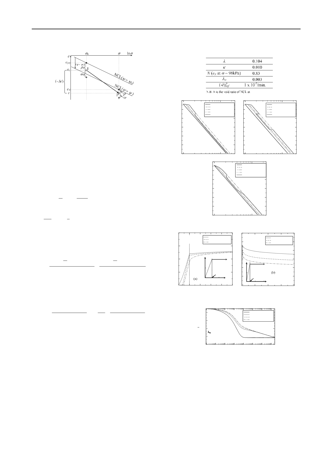
4 SIMULATIONS OF TIME-DEPENDENT BEHAVIOR
4.1
Analysis of normally consolidated clay by three models
Table 1 shows material parameters for Fujinomori clay, which
are common to the three models. The initial rate of plastic void
ratio change is assumed as
0
( ) ( )
p
p
ref
e
e
=1.0x10
-7
/min.
Linear increasing functions,
G
(
)=100
and
Q
(
)=40
, are
employed for the case to consider density and bonding effects.
Figure 6 shows the results of one-dimensional compression
behavior of normally consolidated (NC) clay for different strain
rates, arranged in terms of the
e
-log
relation. In the figure, the
solid straight lines (no creep) show the relation without time
effect, and the thick lines show the results in which strain rate
decreases and increases again along the way. In every model,
the lines of constant strain rate are parallel to each other, which
is a good agreement with published experimental results (e,g.,
Bjerrum, 1967). It is also seen that when the strain rate
decreases at a certain point, the curve follows exactly the same
path which is supposed to follow for the new strain rate.
However, when the strain rate increases again to the previous
rate, the result of the non-stationary flow surface model does
not return to the target curve corresponding to the respective
strain rate which is called the phenomenon of
‘
isotach
e’
. The
result of the over-stress model shows sudden change of stress,
Figure 5. Explanation of the proposed model
Table 1. Material parameters for clay
( ) ( )
p
p
ref
e
e
10
2
10
3
0.55
0.6
0.65
0.7
0.75
0.8
0.85
e
(kPa)
no creep
0.002%/min
0.02%/min
2.0%/min
2.0 - 0.002 - 2.0%/min
Ideal - Drained
=0.0030
(a) Non-stationary
flow surface
10
2
10
3
0.55
0.6
0.65
0.7
0.75
0.8
0.85
e
(kPa)
no creep
0.002%/min
0.02%/min
2.0%/min
2.0 - 0.002 - 2.0%/min
Ideal - Drained
=0.0030
(b) Over-stress
10
2
10
3
0.55
0.6
0.65
0.7
0.75
0.8
0.85
no creep
0.002%/min
0.02%/min
2.0%/min
2.0 - 0.002 - 2.0%/min
Ideal - Drained
e
=0.0030
0
=0.0
0
=0.0
(kPa)
(c) Proposed
Figure 6. Simulations of strain rate effect of NC clay
0
1
2
3
4
5
0
1
2
3
4
(%)
Time (min)
Ideal - Drained
Proposed Model
Sekiguchi 1D Model
Overstress 1D Model
=0.0030
0
=98kPa
=98kPa
(1 minute)
1 2
t
(min)
200
(kPa)
0 100
0
100
200
300
400
100
120
140
160
180
200
220
(kPa)
Time (min)
Ideal - Drained
=0.0030
Proposed Model
Sekiguchi 1D Model
Overstress 1D Model
0
=98kPa
(4 minutes)
10
20
t
(min)
2
1
(%)
00
Figure 7. Simulations of creep and stress relaxation of NC clay
10
-3
10
-2
10
-1
1 10 10
2
10
3
10
4
0.74
0.76
0.78
0.8
0.82
no creep
Proposed Model
Sekiguchi 1D Model
Overstress 1D Model
e
t (min)
=98kPa
=98kPa
H=1cm
=0.0030
Figure 8. Simulations of oedometer test on NC clay


