256
Proceedings of the 18
th
International Conference on Soil Mechanics and Geotechnical Engineering, Paris 2013
Proceedings of the 18
th
International Conference on Soil Mechanics and Geotechnical Engineering, Paris 2013
indicate the initial (
=
0
,
e
=
e
0
) and the current (
=
,
e
=
e
)
states, respectively. The plastic change in void ratio from the
initial state to the current state can be expressed by
0
0
0
0
(
)
( )
ln
( )
ln
where,
(
)ln
( )
p
e
p
p
t
e e e
e F
t
e
F
F
e
(1)
Here,
and
denote compression and swelling indices. By
solving this ordinary differential equation with variables of time
and plastic void ratio change (plastic strain), the plastic change
in void ratio is given in the following form as a function of
stress term
F
and time
t
(Sekiguchi 1977):
0
0
( )
(
)
ln
exp
1
( )
ln
where,
exp
1
p
p
p
e t
F
e
e t
F
S
S
(2)
Then, the increment of plastic void ratio is calculated as
(
)
(
)
( )
1 1
1 1
(
) 1
1
p
p
p
e
e
d e
d
dt
t
d
dt
S
S t
(3)
The elastic increment of plastic void ratio change is given by
1
( )
e
d e
d
(4)
Total increment is given by a summation of the plastic
component of Equation (3) and the elastic component of
Equation (4). As is seen from Equation (3), the non-stationary
flow surface model contains time variable
t
, which is not
objective. The multi-dimensional model in which the stress term
F
is replaced by the yield function of the Cam clay using (
p
,
q
)
corresponds to so-called Sekiguchi model (1977).
2.2
Over-stress type model
As is seen from Figure 3, viscoplastic strain rate of the Bingham
body is given by
1
1
p
c
c
c
(5)
Here, the symbol < > denotes the Macaulay bracket, i.e.
A
=
A
if
A
>0; otherwise
A
=0, and
c
and
are the yield stress and
the coefficient of viscosity. The over-stress type of
viscoplasticity gives the viscoplastic strain rate as follows
generalizing the Bingham viscosity:
( )
where
( )
( ) if >0,
( ) 0 if
0
p
(6)
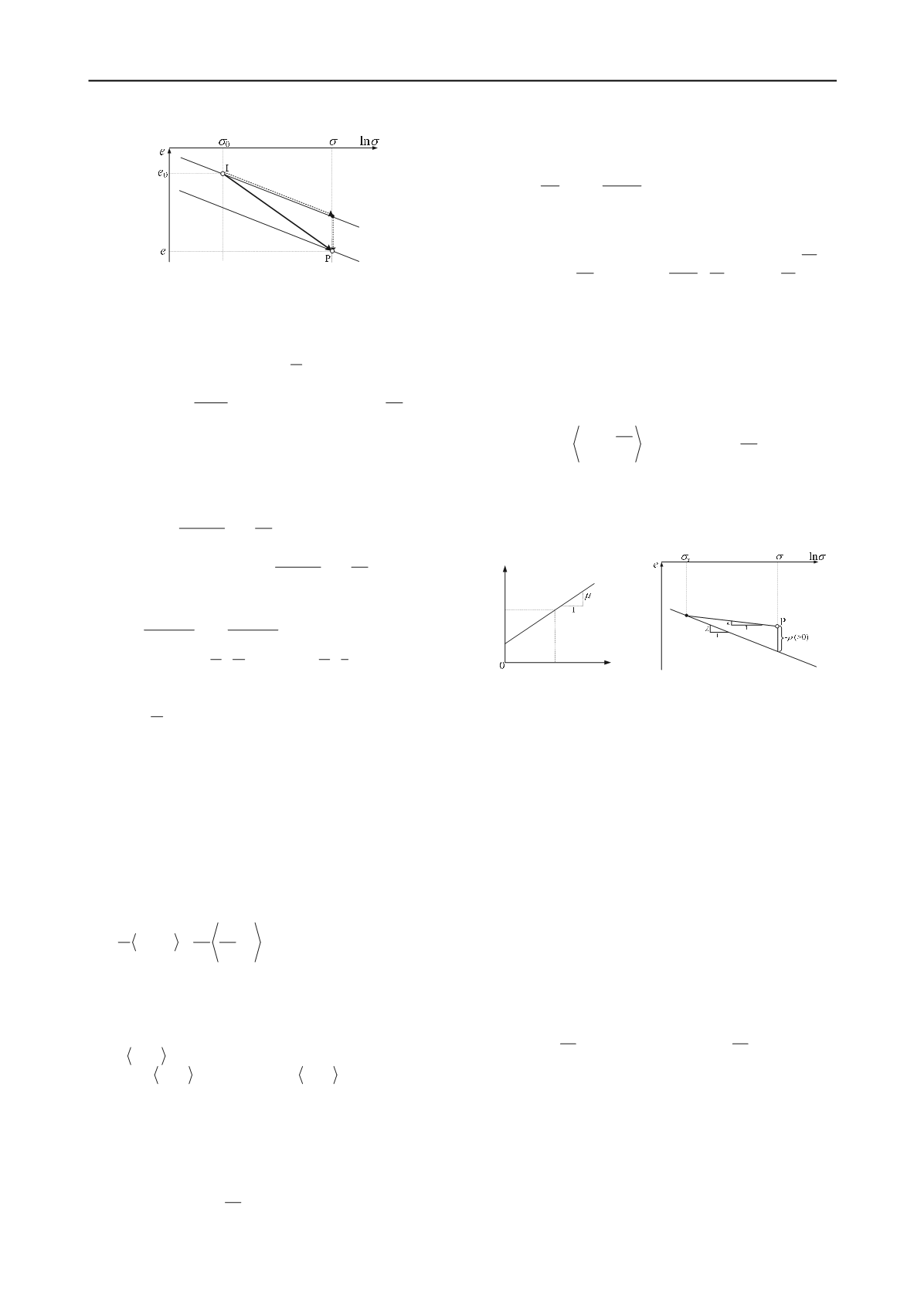
The straight line with slope of
in Figure 4 indicates NCL at
reference state in which the strain rate is sufficiently small. The
condition on this line is called “static”. Now, it is assumed that
clay at point P in Figure 4 satisfies the creep behavior in Figure
1. From Figure 4, the difference between the current void ratio
and that on NCL (-
) at the same stress is expressed as
(
)ln
ref
s
e e
(7)
Also, the following equation is obtained from the interpolated
diagram in Figure 1:
( )
ln
ln
( )
p
ref
p
ref
t
e
t
e
(8)
From Eqatoins (7) and (8), the rate of plastic void ratio change
is expressed as
( ) ( ) exp
( ) exp
ln ( )
p
p
p
p
ref
ref
ref
s
s
e
e
e
e
(9)
Here, the current stress
is called “dyanamic stress”, and the
stress which is determined from the current void ratio
s
is
called “static stress”. These correspond to “dynamic yield
function” and “static yield function” in multi
-dimensional over-
stress type vicsoplastic model. If it is assumed that Equation (9)
holds not only under creep condition but also under other
conditions, the increment of plastic void ratio change is given
by
( ) ( )
1
where = 1
p
p
ref
s
d e
e
dt
(10)
The elastic component is given by Equation (4). it is also
shown by Mimura and Sekiguchi (1985) that Equation (10)
corresponds to Equation (3) in which the term of stress
increment is eliminated. Since the plastic strain increment is
related with time alone, there is no loading condition in this type
of models.
3 NEW TYPE OF TIME-DEPENDENT MODEL
As mentioned above, NCL shifts depending on the strain rate.
The two straight lines in Figure 5 indicate NCLs corresponding
to the initial state (point I;
=
0
,
e
=
e
0,
0
( ) ( )
p
p
e
e
) and the
current state (point P;
=
,
e
=
e
,
( ) ( )
p
p
e
e
). The difference
of these two lines are expressed as (
-
0
). To model not only
normally consolidated clay but also over consolidated clay, the
state variable
(=
e
N
-
e
) which is the difference between the
current void ratio and that on NCL is introduced. Furthermore,
to describe the behavior of structured clay such as naturally
deposited clay, another state variable
, which represent an
imaginary increase of density due to bonding effect, is
employed. In the case of
=0 and
=0, Figure 5 results in
Figure 2. From Figure 5, the plastic change of void ratio is
expressed as
0
0
0
0
0
0
0
ln
ln
p
e
e
N N
e
e
e
e e
e
(11)
Denoting
0
(
)ln( / )
F
in the same way as Equation
(1) and
H
=(-
e
)
p
, the following equaton (1D yield function) is
obtaied:
0
0
(
) (
) 0
f F H
(12)
From the consitency condition (
df
= 0),
0
df dF dH d d
(13)
Now, it can be considered that the evolution rule of
with the
development of plastic deformation for structured soil is
determined not only by the state variable
related to real
p
c
p
Figure 3. Bingham body
0
NCL;
(
)
(
)
p
p
e
e
NCL;
(
)
(
)
p
p
e
e
Figure 2. Explanation of non-stationary flow surface model
NCL ; (
)
(
)
p
p
ref
e
e
Figure 4. Explanation of over-stress
type model


