2883
Technical Committee 212 /
Comité technique 212
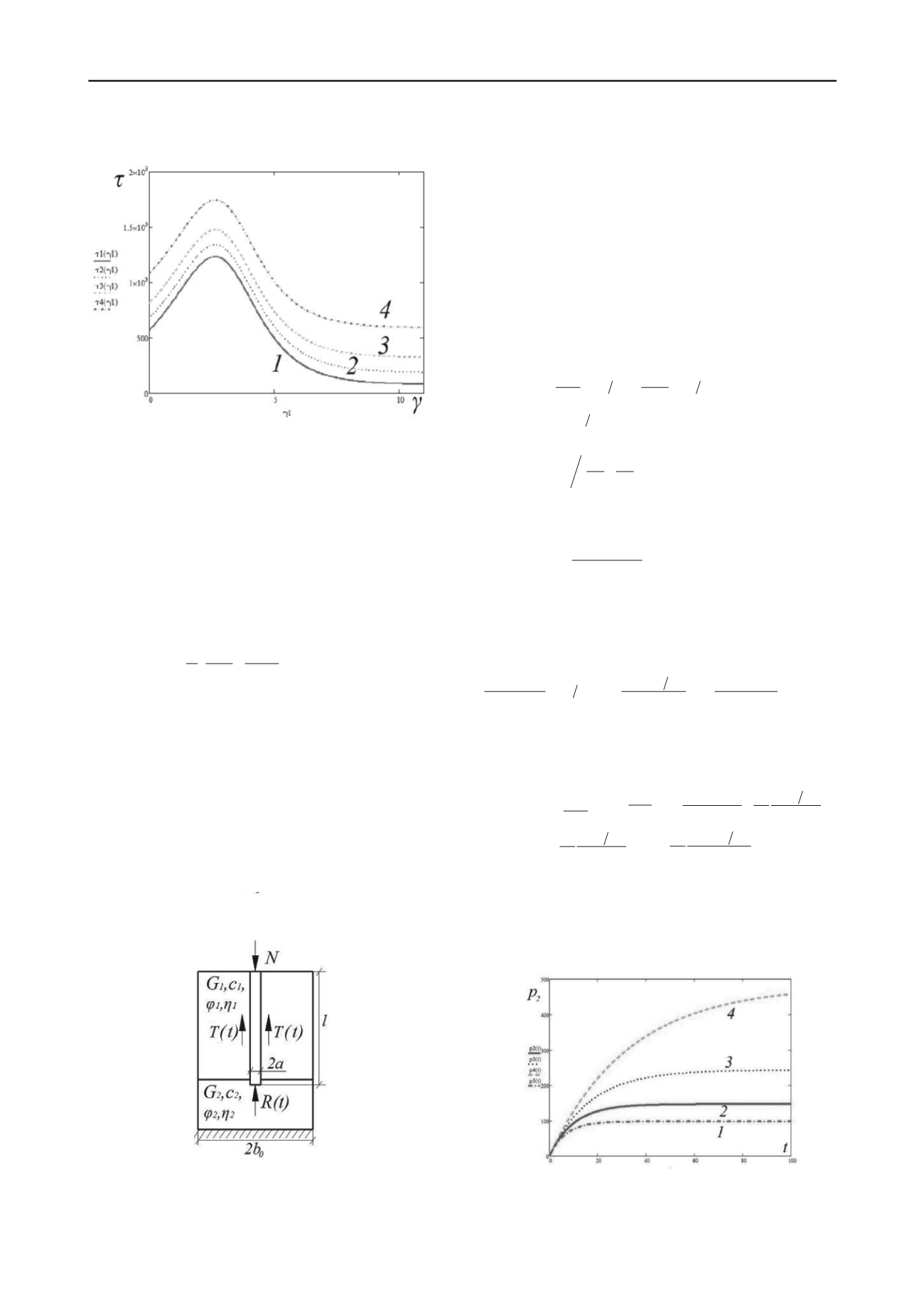
Fig. 4. Curves of
τ
(kPa), depending on
γ (%)
, in kinematic
loading
at various values of compacting loading
σ
(7)
and
σ
1
> σ
2
> σ
3
> σ
4
const
4 STRESS RELAXATION
Equation (1) demonstrates a stress relaxation process
for
0
0
0
i.e., with
and with initial
and
const
t
0
const
*
t
)(
. Solution (1) in this case looks, as
follows:
At
At
e
e
t
0
res
1
(9)
with
b
e
a
eGA
0
0
,
(10)
th,
p
1
,
p
2
as stresses at pile
ead and und
and 2-
rs of
deformation, strength and viscosity respectively
f
res
τ
as residual strength
res
Let us determine the limit curve of residual strength
from relaxation curves for different values of compressive
stresses
σ
(see Fig.1, c, on the left side).
5 SOME PROBLEMS OF APPLIED SOIL MECHANICS
The problem of a pile interaction with rheological soil
can be reduced to determining regularities of constant force
N
distribution between side resistance and bottom resistance
(fig.5) and
)( )(
tT tRN
with
i
,
,
2
,
a
0
,
b
0
as pileradius and
pile influence area;
l
as pile leng
pa N
2
0
la T
2
0
2
2
0
pa R
h
er its tip respectively.
Fig.5 Principal schematic of interaction between pile
layer soil massive, where
G, φ, c
и
η
are paramete
In order to solve this problem the pile settlements,
caused by forces
T(t)
and , shall be calculated and then
related to the pile deformation modulus
E
p
that is much greater
than the surrounding soil modulus
E
s
i.e.,
E
p
>>
E
s
. Consider
various cases of bi-layer soil with upper layer, having
viscoelastic properties as in eq. (4) while the lower one being
elastic, viscoelastic, elastic-plastic and viscous.
)(
tR
5.1
Linear deforming soil under pile tip
Let us determine pile settlement rate due to friction
from solution, based on the assumption for the shear mechanism
of soil displacement around pile with volume deformations
being neglected [11]. For
)(
tT
0
*
0 0
1
0
0 0
1
ln
ln
ab
tG
a ab
t
a S
a
a
T
(12)
with
al
T
a
2
and
as pile settlement rate. -
rate of changing
T
S
а
а
1
1
1
1
1
1
( )
(
)
t
t
e e
t
a b
(13)
The rate of settlement, generated by force is also
determined from solution for a circular stiff plate, pressed in
elastic medium
)(
tR
2
1 2 0
2
4
1
G
K
a p S
T
(14)
With
as coefficient, accounting for the depth of
load application to the plate;
и
- applied stress and rate
of its changing.
1 )(
lK
2
p
2
p
By comparing eq. (12) and eq. (14) with the account of
eq. (11) we obtain:
2
1
2
2
1
0 0
2
0
2 0 0
1
2 1
2
0
4
1
2
ln
ln
2
G
K a p
lG
ab a p ab
t l
p p a
(15)
After some transformations we get the following
differential equation:
2
2
1
( )
( )
p p P t
p Q t
(16)
with
( )
( )
B t
P t
A
,
A
tD tQ
;
1
0 0 0
2
1
2
ln
2
4
1
G
ab
l
a
G
K
A
;
t
ab
l
a tB
1
0 0 0
ln
2
;
t
ab p
l
a tD
1
0 0 1 0
ln
2
(17)
Solution (16) for initial condition
, obtained
with the help of MathCad software, yielded that
p
2
varies versus
time with different rates and tends to constant values (Fig. 6).
The pile settlement is also determined from eq, (14), by
introducing
instead of
.
0 )0(
2
p
)(
2
t p
)(
2
t p
(a)
Fig. 4. Curves of
τ
(kPa), depending on
γ (%)
, in kinematic
loading
at various values of compacting loading
σ
(7)
and
σ
1
> σ
2
> σ
3
> σ
4
const
4 STRESS RELAXATION
Equation (1) demonstrates a stress relaxation process
for
0
0
0
i.e., with
and with initial
and
const
t
0
const
*
t
)(
. Solution (1) in this case looks, as
follows:
At
At
e
e
t
0
res
1
(9)
with
b
e
a
eGA
0
0
,
(10)
th,
p
1
,
p
2
as stresses at pile
ead and und
and 2-
rs of
deformation, strength and viscosity respectively
f
res
τ
as residual strength
res
Let us determi e the limit curve of residual strength
from relaxation curves for different values of compressive
stresses
σ
(see Fig.1, c, on the left side).
5 SOME PROBLEMS OF APPLIED SOIL MECHANICS
The problem of a pile interaction with rheological soil
can be reduced to determining regularities of constant force
N
distribution between side resistance and bottom resistance
(fig.5) and
)( )(
tT tRN
with
i
,
,
2
,
a
0
,
b
0
as pileradius and
pile influence area;
l
as pile leng
pa N
2
0
la T
2
0
2
2
0
pa R
h
er its tip respectively.
Fig.5 Principal schematic of interaction between pile
layer soil massive, where
G, φ, c
и
η
are paramete
5.1
Linear deforming soil under pile tip
Let us determine pile settlement rate due to friction
from solution, based on the assumption for the shear mechanism
of soil displacement around pile with volume deformations
being neglected [11]. For
)(
tT
0
*
0 0
1
0
0 0
1
ln
ln
ab
tG
a ab
t
a S
a
a
T
(12)
with
al
T
a
2
and
as pile settlement rate. -
rate of changing
T
S
а
а
1
1
1
1
1
1
( )
(
)
t
t
e e
t
a b
(13)
The rate of settlement, generated by force is also
determined from solution for a circular stiff plate, pressed in
elastic medi m
)(
tR
2
1 2 0
2
4
1
G
K
a p S
T
(14)
With
as coefficient, accounting for the depth of
load application to the plate;
и
- applied stress and rate
of its changing.
1 )(
lK
2
p
2
p
By comparing eq. (12) and eq. (14) with the account of
eq. (11) we obtain:
2
1
2
2
1
0 0
2
0
2 0 0
1
2 1
2
0
4
1
2
ln
ln
2
G
K a p
lG
ab a p ab
t l
p p a
(15)
After some transformations we get the following
differential equation:
2
2
1
( )
( )
p p P t
p Q t
(16)
with
( )
( )
B t
P t
A
,
A
tD tQ
;
1
0 0 0
2
1
2
ln
2
4
1
G
ab
l
a
G
K
A
;
t
ab
l
a tB
1
0 0 0
ln
2
;
t
ab p
l
a tD
1
0 0 1 0
ln
2
(17)
Solution (16) for initial condition
, obtained
with the help of MathCad software, yielded that
p
2
varies versus
time with different rates and tends to constant values (Fig. 6).
The pile settlement is also determined from eq, (14), by
introducing
instead of
.
0 )0(
2
p
)(
2
t p
)(
2
t p
(a)
Fig. 4. Curves of
τ
(kPa), depending on
γ (%)
, in kinematic
loading
at various values of compacting loading
σ
(7)
and
σ
1
> σ
2
> σ
3
> σ
4
const
4 TR SS RELAXATION
Equation (1) demonstrat s a stress relaxati n process
for
0
0
0
i.e., with
and with initial
and
cons
t
0
const
*
t
)(
. Solution (1) in this case looks, as
follows:
At
At
e
e
t
0
res
1
(9
with
b
e
a
eGA
0
0
,
(10)
th,
p
1
,
p
2
as stresses at pile
ead and und
and 2-
rs of
deformation, strength and viscosity respectively
f
res
τ
s resid al strength
res
Let us determine the lim t curve of residual strength
from relaxation curves for different values of compressive
stresses
σ
(see Fig.1, c, on the left side).
5 SOME PROBLEMS OF APPLIED SOIL MECHANICS
The probl m of a pil nteractio with rheological soil
can be reduced to determining regularities of constant force
N
distribution between side resistance and bottom resistance
(fig.5) and
)( )(
tT tRN
with
i
,
,
2
,
a
0
,
b
0
as pileradius and
pile influence area;
l
as pile leng
pa N
2
0
la T
2
0
2
2
0
pa R
h
er its tip respectively.
Fig.5 Pri cipal schematic of interaction between pile
layer soil massive, where
G, φ, c
и
η
are paramete
In order to solve this problem the pile settlements,
caused by forces
T(t)
and , shall be calculated nd th n
related to th pile deformation modulus
E
p
that is much greater
than the surr unding soil modulus
E
s
i.e.,
E
p
>>
E
s
. Consider
v rious cas s of bi-layer oil with upper layer, having
viscoelastic properties as in eq. (4) while the lower one being
elastic, viscoelastic, elastic-plastic and viscous.
)(
tR
5.1
Linear deforming soil under pile tip
Let us det rmine pile settlement rate due to friction
from solution, based on th assumption for the shear mechanism
of soil displacement around pile with volume deformations
being neglected [11]. For
)(
tT
0
*
0 0
1
0
0 0
1
ln
ln
ab
tG
a ab
t
a S
a
a
T
(12)
with
al
T
a
2
and
as pile settlement rate. -
rate of changing
T
S
а
а
1
1
1
1
1
1
( )
(
)
t
t
e e
t
a b
(13)
The rate of settlement, generated by force is also
determined from solution for a circular stiff plate, pressed in
elastic medium
)(
tR
2
1 2 0
2
4
1
G
K
a p S
T
(14)
With
as coefficient, accounting for the depth of
load application to the plate;
и
- ap lied stress and rate
of its changing.
1 )(
lK
2
p
2
p
By comparing q. (12) and eq. (14) with the account of
eq. (11) we obtain:
2
1
2
2
1
0 0
2
0
2 0 0
1
2 1
2
0
4
1
2
ln
ln
2
G
K a p
lG
ab a p ab
t l
p p a
(15)
After some transformations we get the following
differential equation:
2
2
1
( )
( )
p p P t
p Q t
(16)
with
( )
( )
B t
P t
A
,
A
tD tQ
;
1
0 0 0
2
1
2
ln
2
4
1
G
ab
l
a
G
K
A
;
t
ab
l
a tB
1
0 0 0
ln
2
;
t
ab p
l
a tD
1
0 0 1 0
ln
2
(17)
Solution (16) for initial condition
, obtained
with the help of Ma hCad softwar , yielded that
p
2
varies versus
time with different rates and tends to constant values (Fig. 6).
The pile settlement is also determined from eq, (14), by
introducing
instead of
.
0 )0(
2
p
)(
2
t p
)(
2
t p
(a)


