2882
Proceedings of the 18
th
International Conference on Soil Mechanics and Geotechnical Engineering, Paris 2013
While summarizing these investigations S.S. Vyalov [1]
emphasized that soil creep is accompanied by mutually opposite
events of soil hardening and softening. If hardening dominates,
then it leads to decreasing of deformations, if softening then it
leads to failure. And he developed a kinematic theory of soil
str
uation bel
isco-plastic strain
rates i.e.,
where vis ity and cohesion variation
rates e
(1)
1.2
witha ,b ,
ength and creep, based on Ya.I.Frekel molecular theory of
soil flow.
The eq
ow relates to the flow theory, in which
strain rate isthe sum of elastic
e
and v
vp e
vp
rsus time are taken
cos
v
into account:
,
as strengthening a
p
(2)
i
Consider rheological
2 CREE
on
ee Fig.1 а, top portion) the critical
nd softening
*
arameters, G as shear modulus;
as creep threshold:
tc tg
` *
with σ` as effective stress, с(t) as time dependent
cohesion.
For triaxial compression eq. (1) looks similar if index i
is added to all parameters that means transfer to strain rates
γ
due to shear stresses
,
*
and
σ`
.
i
i
processes on the basis of eq. (1) below.
P AND LONG-TERM STRENGTH
Analysis of eq. (1) with constant cohesion ratio
(
const
tc
)(
) and volume deformati showed that at flexure
points of creep curves (s
values of
, based on condition
cr
0
, are constant and are
described by equations as
const
a
cr
ln 1
(3)
b
ce, ea
.T
parameters of creep curves, yield long-
zing laboratory test data. In
order to describe creep in soil mass asin (1) the following
equation can be applied:
with respective stresses
τ
cr
(γ
cr
)
depend on applied
τ
и
γ
cr
,
i.е.,
) ,(
cr
cr
f
,
) ,(
cr
cr
f
t
.
The creep curve flexure time point
t
п
can be determined
from the curve (see Fig. 1) i.e., from the crossing points of lines
γ(t)
and
γ
cr
=
const. Hen ch
τ
corresponds to
τ
cr
and
t
cr
hus,
(1) and (3), based on
term strength curve
) (
nn
t
, using parameters τ
0
and
(see
Fig. 1a, bottom part).
Eq. (1) can be used for analy
G b
e
a
e
t
t
1
1
*
1
1
(4)
If
const
:
1
1
1
1
b
e
a
e
(5)
*
t
t
Solution (5) can be expressed as follows:
11 11
1
1
*
b
e
a
e
t
t
t
G b a t
)(
*
e e
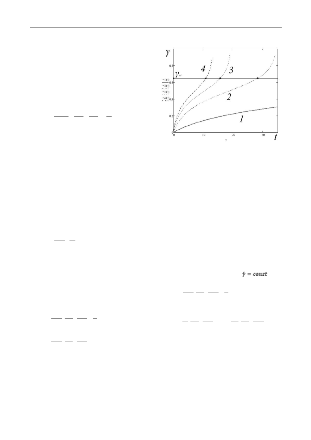
Fig. 3. Curves
γ
(in decimals) and
t
(in hours) for clay
soil with different values of tangential stresses in simple shear
conditions, according to eq. (1) with known parameters
α,β, a
,
b
и
η
and
τ > τ
*
,
τ
1
< τ
2
<
τ
3
<
τ
4
Calculation as per (5) demonstrates that dependence
γ(t)
features double curvature same as in case (1) i.e., depending on
the level of stress
, and parameters ,
b
1
, , that depict
decaying, non-decaying and progressive creep (Fig. 3). Such
result is due to the difference of exponential functions in
brackets in eq. (4), the first of which describes strengthening
while the second relates to softening.
1
a
1
1
Eqs. (1) and(5) are identical, as they give the same
results.In order to apply eq. (5) for solving boundary problems
it is necessary to determine parameters ,
b
1
,
,
from
experiments that can differ from parameters in Eq.(1).
1
a
1
1
3 KINEMATIC SHEAR
Soil sample deviator loading is a broadly applied triaxial
test, following hydrostatic compression with constant axial
deformation rate
. In simple shear (distortion) under
kinematic loading (
const
1
const
) eq. (1) with
looks,
as follows:
G b
e
a
e
vt
vt
*
(7)
with
v
as angular strain rate
const
v
We obtain from eq. (7)
b
e
a
eG Gv
b
e
a
eG
vt
vt
vt
vt
*
(8)
Solution of this differential equation, obtained
numerically with the help of MathCad software for various
shear strain values
, enablesplotting a family of curves
τ(t) - γ
(Fig. 4). The calculations showed that they haveextreme
points at characteristic time
t
cr
=const and acommon asymptote.
It is obvious thatfrom those curves wecan plotcurves
τ
max
(σ)
и
τ
min
(σ)
in case of
.
n
...
,
2 1
const
(6)


