2450
Proceedings of the 18
th
International Conference on Soil Mechanics and Geotechnical Engineering, Paris 2013
where
z
= the spatial coordinate;
t
= time;
u
= the excess pore
water pressure;
c
v
= the coefficient of consolidation of the soil;
p
vac
= the magnitude of the applied vacuum pressure at
z
= 0;
and
H
is the thickness of the deposit.
With the presence of a vacuum pressure, the final state is not a
condition with zero excess pore pressure in the deposit.
Therefore, the solution to the governing equation must consist
of two parts, namely the steady state solution (
Y
(
z
)) and the
transient solution (
v
(
z,t
)) (Chai and Carter 2011). With the
boundary condition defined by Eq. (2),
u
(
z
,
t
) can be expressed
in the following form:
),(
),(
)(
),(
2
1
tzvp tzvp zYp tzu
s
vac
vac
(4)
where
p
s
= the magnitude of the applied surcharge load. The
term -
p
vac
Y
(
z
) is the final steady state excess pore water pressure
distribution and (
p
vac
v
1
(
z
,
t
)+
p
s
v
2
(
z
,
t
)) is the time-dependent
component of the excess pore water pressure.
2.1.1
One-way drainage
For this case the excess pore water pressure distribution is given
by:
1
2
sin
1 2
1 4 )
(
n
tca
n
s
vac
vac
vn
eza
n
p p p u
(5)
where
a
n
= (2n-1)
π
/(2
H
). In this case,
Y
(
z
) = 1, and the
v
1
(
z
,
t
) =
v
2
(
z
,
t
) and its expression is given in the last set of parentheses
of Eq. (5). The average degree of consolidation is given by:
1
1 2
4
2
2
2 2
2
1 2
1
8 1
n
n
H
tc
v
e
n
U
(6)
2.1.2
Two-way drainage
In this case the excess pore water pressure distribution in the
soil is given by:
1
2
)
(
sin
sin
2
1
),(
n
tc
n
s
n
s
vac
vac
vn
e
zH
n
p
z
n
p p
H
z
p tzu
(7)
where
Hn
n
. The average degree of consolidation is
given by:
1
1 2
2
2
2 2
2
1 2
1
8 1 )(
n
n
H
t c
vs
e
n
tU
(8)
2.2
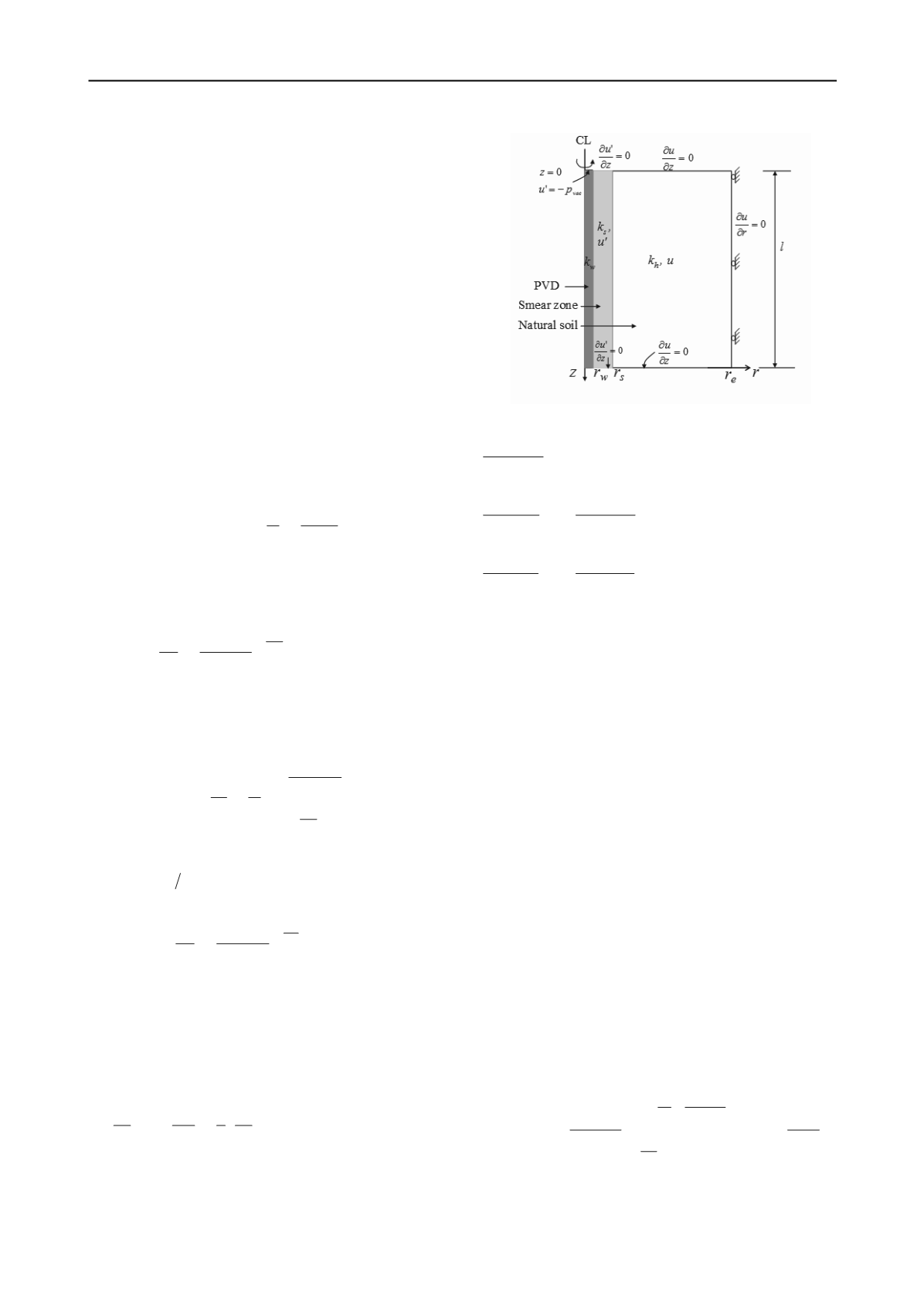
Uniform layer with PVD improvement
The theory for a PVD-improved soil deposit is derived here for
the case of one-way drainage conditions using a unit cell model,
as shown in Fig. 1. The governing equation for consolidation is
as follows:
r
u
r
r
u c
t
u
h
1
2
2
(9)
where
r
= the radial distance and
c
h
= the coefficient of
consolidation in the horizontal direction. The boundary
conditions are:
Figure 1. Unit cell model and boundary conditions
0 , ,
r
tzru
e
(10)
0 ,0,
z
t ru
,
0 ,0, '
z
t ru
(11)
0 ,,
z
tlru
,
0 ,, '
z
tlru
(12)
vac
w
p t r u
,0,
'
(13)
where
u
and
u
' = the excess pore water pressures in the
undisturbed zone and the smear zone, respectively (Fig. 1),
z
=
depth from the ground surface,
r
w
= equivalent radius of a PVD,
and
r
e
= radius of the unit cell. The solutions for
u
and
u
' can be
expressed as:
), ,()
(
), ,(
tzrvp p p tzru
s
vac
vac
for (
r
s
<
r
r
e
) (14)
), ,(')
(
), ,('
tzrvp p p tzru
s
vac
vac
for (
r
w
<
r
r
s
) (15)
where
r
s
= radius of the smear zone. The additional conditions
for getting explicit expressions for
v
and
v
' are the following
water flow continuity conditions.
(1) The total inflow of pore water through the boundary of a
cylinder with a radius of
r
has to be equal to the change in
volume of the hollow cylinder with outer radius of
r
e
and
inner radius of
r
.
(2) The pore water flow into the PVD from a horizontally cut
soil slice is equal to the change of vertical flow rate in the
PVD.
At the interface between the smear zone and the undisturbed
zone, the radial flow rate from the undisturbed zone is equal to
the flow rate into the smear zone.
With these conditions and using the same assumptions as
those adopted in obtaining Hansbo’s (1981) solution, it can be
shown that the expressions for
v
(r,
z
,
t
) and
v
′(r,
z
,
t
) are as
follows:
h
w
s
w
w
e
e s
h
T
z lz
n
k
k
r r
r
r r
r k
k
tzrv
8 exp
21
2
ln
, , '
2
2
2
2
2
2
fo
r (
s
w
r r r
)(16)


