2202
Proceedings of the 18
th
International Conference on Soil Mechanics and Geotechnical Engineering, Paris 2013
Z
Y
X
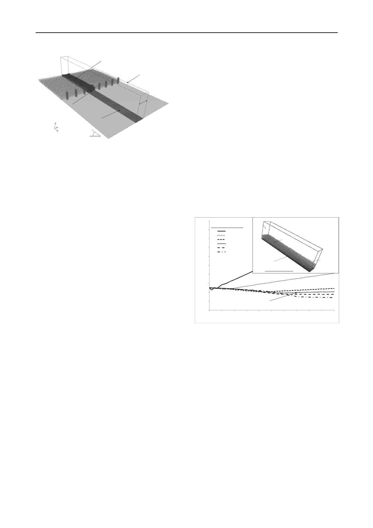
Initial position of the granular material. The
flow depth is uniform.
Computation domain
Flow path
An infinite array of baffles was simulated
by repeating the computation domain
using periodic boundary condition
35
0
1.2m
Figure 1. Numerical model setup
The length and width of the computation domain were 15m and
1.2m respectively. The slope gradient was chosen to be 35
0
.
The plan area and the height of the individual baffle were 0.2m
x 0.2m and 1m respectively. The baffle was located in the
middle of the flow path. The periodic boundary condition (PBC)
was applied along the y-direction (Figure 1) of the computation
domain. With the PBC, discrete elements leaving one side of
the computation domain in the y-axis will emerge on the
opposite side with the same dynamic properties, such as
velocity, force, etc. This boundary condition helps to reduce the
computation time since the impact of granular flow medium on
an array of baffles could be simulated using a single baffle and a
reduced number of discrete elements (i.e. only the dark particles
shown in Figure 1 need to be modelled). With reference to
Chen 2009, a baffle spacing of 1m and the ratio of baffle
spacing to element diameter of 20 were adopted in the analysis
to prevent clogging of the discrete elements between the baffles.
Each numerical analysis is divided into two stages, namely
the initial stage and the impact stage. At the initial stage, the
granular medium comprising an assembly of discrete elements
with random packing was placed on a rigid surface inclined at
35
0
as shown in Figure 1. The individual discrete elements
stabilized itself under the action a body force, which was
equivalent to gravity and acting perpendicularly downwards at
the ground surface. The body force acting on the individual
discrete elements was rotated to the vertical direction in the next
stage to enable the granular medium to flow downslope under
the action of gravity and impact the baffles. The initial
thickness of the granular medium was uniform and chosen to be
0.5m before impacting on the baffles. At the impact stage, the
granular medium was given an initial velocity of 8 m/s. The
corresponding Froude number of the initial flow condition is
close to 4 which fall within the range of Froude number of
debris flow events reported by Hubl et al 2009.
2.3
Contact law applied in numerical model
The local rheology of the flow material was simulated by
applying the contact law in the numerical model. The linear
Hookean stiffness model was adopted for the discrete elements
and the rigid planar surfaces in the numerical analyses.
According to Crosta et al. 2001, the contact stiffness of the
discrete element has negligible influence on the computed
mobility of granular material. Given that the chosen stiffness
value have only minimal influence on the computed result, the
discrete element and wall stiffness used were both chosen to be
1x10
8
(N/m) such that the elements almost behave like a rigid
body.
The relative translational and rotational motions between
the discrete elements are mainly resisted by contact friction.
The macroscopic friction angle of dry sand was measured to be
35
0
(Teufelsbauer et al. 2011, Chiou 2005, Pudasaini et al 2005
and 2007, Pudasaini and Hutter 2007). Based on field and
laboratory tests conducted by Chau et al. 2002, Azzoni and
Freitas 1995 and Robotham et al. 1995, the coefficient of
restitution was chosen to be 0.5.
According to Calvetti and Nova 2004, the macroscopic
friction angle of the granular medium is typically much less
than 30
0
irrespective of the value of the contact friction angle
adopted on spherical discrete elements without rolling
resistance. Calvetti et al 2003 and Tamagnini et al 2005
emphasized the need to inhibit particle rotations and calibrate
the particle contact friction angle based on the desired value of
the macroscopic friction angle of the granular medium.
In the numerical analyses, a rolling resistance term was
added in the calculation of rolling motion of discrete elements.
The rolling resistance was calculated using a directional
constant torque model elaborated by Ai et al 2011. The model
applies a constant torque on a particle to represent the rolling
friction. The direction of the torque was always against the
relative rotation between the two contact entities. The torque
between two in-contact spheres i and j can be expressed as:
M
r
=-(
rel
/ |
rel
|)
r
R
r
F
n
(1)
rel
=
i
-
j
(2)
where
ω
i
= the angular velocities of sphere i;
ω
rel
= the relative angular velocity between two elements;
r
= the rolling friction coefficient;
F
n
= the normal contact force; and
R
r
= the radius of the discrete element
0.5
0.7
0.9
1.1
1.3
1.5
1.7
1.9
2.1
2.3
2.5
0
5
10
15
20
25
30
35
40
45
50
Ke / Ke0
Time (s)
0.2
0.4
0.6
0.7
0.8
1
Rolling friction coefficient
The kinetic energy of the discrete elements reaches a steady value when the
rolling friction coefficient equals 0.7.
Channelbed
Periodic boundary
condition
Periodic boundary
condition
Granularmaterial
Directionof flow
Numerical model setup
Figure 2. The effects of the rolling friction coefficient on the time
history of the computed kinetic energy
A calibration exercise was carried out to identify the appropriate
rolling friction coefficient for the numerical study. Figure 2
shows the numerical setup for the calibration work. The
simulation box boundary was periodic in nature in order to
allow the granular material to transport on the incline
indefinitely. The granular material was given an initial velocity
of 8m/s. By adopting a macroscopic friction angle of 35
0
(i.e.
same as the channel inclination), a coefficient of restitution of
0.5 and trying different rolling friction coefficients (i.e.
r
= 0.2,
0.4, 0.6, 0.7, 0.8 and 1) in the calibration exercise, the granular
flow would eventually reach a steady kinetic energy.
Figure 2 shows the time history of the kinetic energy (k
e
) of
all discrete elements relative to the computed k
e
at time zero
(k
e0
). The k
e
is the sum of kinetic energy of all discrete
elements. Based on the results of the calibration exercise, the
granular flow could attain a steady velocity when the rolling
friction coefficient reached a value of 0.7, which was chosen to
be the appropriate rolling friction coefficient for the numerical
study. The input parameters adopted is summarized in Table 1.


