2154
Proceedings of the 18
th
International Conference on Soil Mechanics and Geotechnical Engineering, Paris 2013
state of sands and in situ observations. The key contribution is
the incorporation of a constitutive model with predictive
capabilities for describing transitions from contractive to
dilative volumetric behavior upon shearing. As a result, the
approach is able to distinguish among different types of sand
response induced by an undrained perturbation (e.g., complete
liquefaction, partial liquefaction, etc.), which is an essential
aspect to define the expected post-failure behavior of a sliding
mass.
In order to define in appropriate mathematical terms the
onset of failure in a shallow infinite slope, our methodology
frames static liquefaction within the theory of material stability
[Hill, 1958, Buscarnera et al. 2011, Buscarnera and Whittle
2013]. In particular, we introduce an index for undrained simple
shear failure:
LSS
LSS
H H
Λ = −
(1)
where
H
is the hardening modulus of the sand considered as an
elastoplastic medium, while
H
LSS
is a kinematic correction
factor that depends on the mode of deformation. Vanishing
values of (1) indicate the onset of unstable conditions. In other
words,
H
LSS
represents a critical value of the hardening modulus
at which undrained simple shear perturbations are no longer
admissible. More details about the derivation of the index (1)
are given by Buscarnera and Whittle (2012). For the purpose of
the current paper, it is sufficient to note that positive values of
(1) at a given state of stress and density reflect a stable
undrained response of the infinite slope, while
vanishing/negative values indicate the loss of undrained
strength capacity. In this way, the values of
LSS
Λ
(as well as its
increment,
LSS
Λ
&
) can be used to assess both the initial stability
conditions prior to shearing and the critical triggering
perturbations. More specifically, the simple shear response
predicted by a constitutive model can be interpreted by means
of (1), identifying the stresses at the initiation of a flow failure
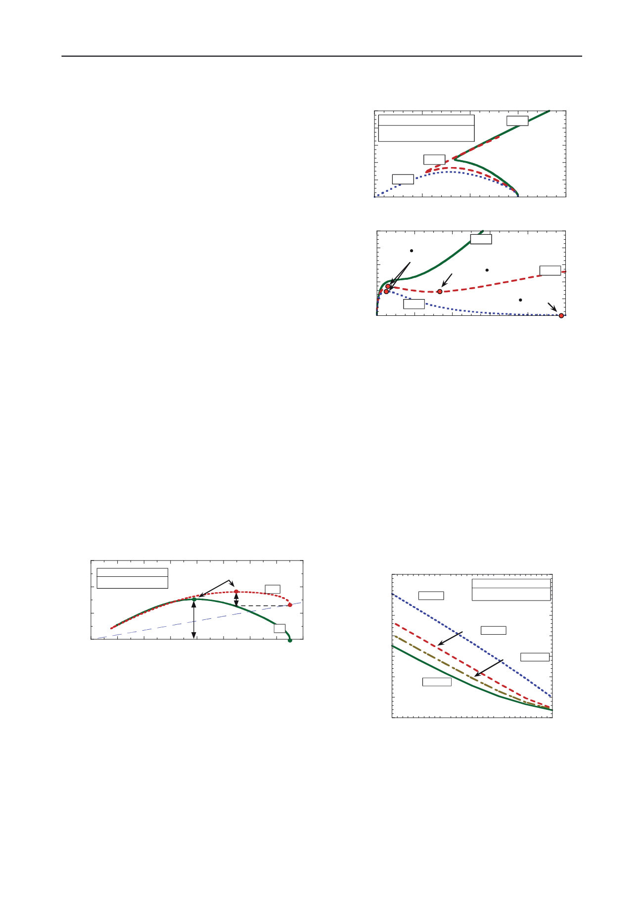
and the residual margin of safety. For example, Figure 2
illustrates two MIT-S1 simulations of undrained simple shear
response at the same level of initial vertical effective stress but
with different values of initial shear stresses (representing
different slope angles).
Figure 2. Example of simple shear simulations (loose Toyoura Sand
simulated with the MIT-S1 model).
The results illustrate that the initial state of stress affects the
magnitude of the shear perturbation required to induce
instability (
∆τ
1
vs
∆τ
2
). The onset of an instability coincides
with the peak in the shear stress, and can be readily interpreted
through the stability index (1).
As is well known, the undrained behavior of sands is also
influenced by changes in the effective stress and density. For
example, even very loose sands can exhibit a tendency to dilate
at low effective stress levels, but will collapse for undrained
shearing at high levels of effective stress. Hence, the prediction
of liquefaction potential requires a constitutive framework that
can simulate realistically the stress-strain properties as functions
of stress level and density. To illustrate this aspect, Figure 3
shows MIT-S1 simulations for a pre-shear void ratio ranging
from 0.87 to 0.94, with the model predicting a sharp transition
from a stable behavior to complete collapse.
Figure 3. MIT-S1 predictions: effect of void ratio on undrained simple
shear response of Toyoura Sand: a) stress path; b) stress-strain behavior.
The effect of confining pressure and density on the
undrained response of sands implies that the perturbation shear
stress ratio,
∆τ
/
σ
’
v0
, associated with the initiation of
liquefaction is not only a function of the slope angle, but must
be evaluated at the depth of interest. This information can be
encapsulated in appropriate stability charts of the triggering
perturbations. Figure 4 gives an example of such charts, and
uses MIT-S1 simulations for a constant value of the initial void
ratio to show the effect of the stress level on the predicted
triggering perturbations.
In general, such charts should be evaluated at any depth of
interest, being they a function of the values of density and stress
state at that specific location. Once the stability charts
expressing the shear resistance potential have been obtained, it
is possible to define the variation of the triggering perturbation
at any depth. These capabilities are illustrated in the next
section by applying the theory for a case study involving flow
failures in a sandy deposit.
Figure 4. Effect of effective stress level on the stability charts (all points
in the chart are characterized by
Λ
LSS
=0).
3 EXAMPLE OF APPLICATION: THE NERLERK CASE.
The Nerlerk berm case history refers to an impressive series
of slope failures that took place in 1983 during construction of
an artificial island in the Canadian Beaufort Sea (Sladen et al.,
1985b). We have used the MIT-S1 model to investigate
potential static liquefaction mechanisms in the Nerlek berm. In
order to apply the theory to the Nerlerk case, it is assumed that
the local behavior of the sides of the berm can be approximated
0
20
40
60
0
20
40
60
80
100
120
140
Shear Stress,
τ
[kPa]
Vertical Effective Stress,
σ
'
v
[kPa]
τ
0
=
σ
'
V
tan
α
∆τ
2
∆τ
1
0°
10°
α
=
MIT-S1: Toyoura Sand
e
0
= 0.93; K
0
= 0.49
Initiation of
liquefaction (
Λ
LSS
=0)
0
20
40
60
80
100
0
50
100
150
200
0.87
e
0
=
0.91
0.94
Shear Stress,
τ
[kPa]
Vertical Effective Stress,
σ
'
v
[kPa]
MIT-S1: Toyoura Sand
σ
'
v0
= 150kPa; K
0
= 0.49
0
2
4
6
8
10
0
20
40
60
80
100
0.87
e
0
=
0.91
0.94
Shear Strain,
γ
(%)
Inception of
instability
(
Λ
LSS
=0;
Λ
LSS
<0)
Quasi steady state
(
Λ
LSS
=0;
Λ
LSS
>0)
Ultimate steady state
(
Λ
LSS
=0;
Λ
LSS
=0)
Shear Stress,
τ
[kPa]
0
5
10
15
0
0,05
0,1
0,15
0,2
0,25
0,3
0,35
MIT-S1: Toyoura Sand
e
0
= 0.93; K
0
= 0.49
15 kPa
σ
'
v0
=
75 kPa
σ
'
v0
=
150 kPa
σ
'
v0
=
300 kPa
σ
'
v0
=
Slope Inclination,
α
[°]
Perturbation Shear Stress Ratio,
∆τ
/
σ
'
V0


