1665
Technical Committee 203 /
Comité technique 203
Proceedings of the 18
th
International Conference on Soil Mechanics and Geotechnical Engineering, Paris 2013
3
4 RESULTS
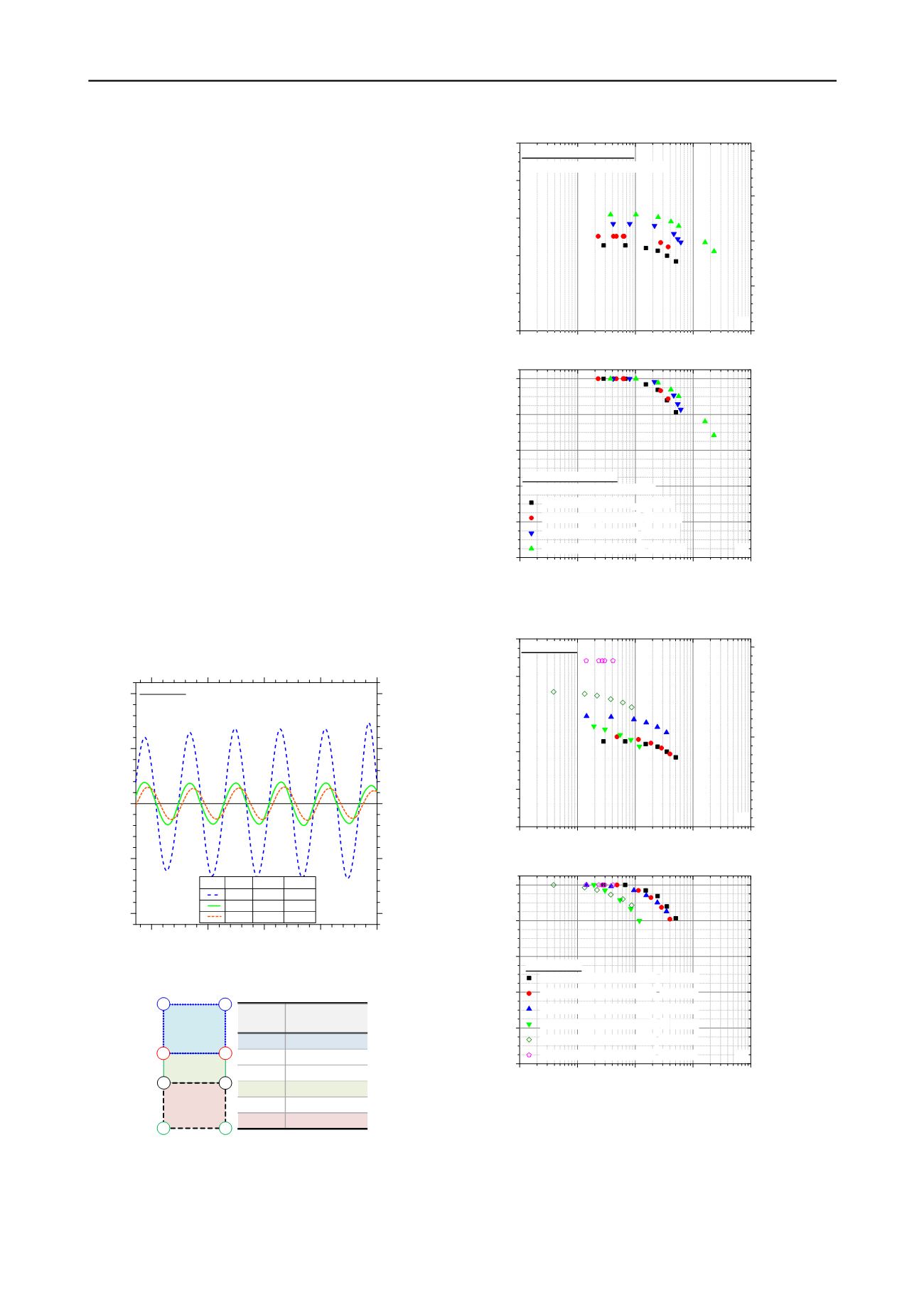
The effect of confining stress on the shear modulus and the
normalized shear modulus as a function of shear strain are
shown in Fig. 7a and 7b, respectively. The impact of waste
composition is eliminated by examining the same set of four
geophones. Example results are shown for element A, i.e., the
set of geophones nearest to the foundation. As shown in Fig. 7a,
G
max
increases from 23 MPa to 31 MPa, as average confining
stress increases from 14 kPa to 89 kPa. In addition, the
G
/
G
max
curve (Fig. 7b) systematically moves to the right, i.e., exhibits a
more linear response with increasing confining stress. These
trends are consistent with laboratory studies on MSW (Lee
2007, Zekkos et al. 2008, Yuan et al. 2011).
The estimated shear modulus reduction and normalized shear
modulus reduction as a function of strain for different sets of
geophones (i.e., elements) are shown in Fig. 8. Data shown in
Fig. 8 are representative of essentially the same confining stress
(11-14 kPa). Elements A, D and F are representative of waste at
different depths. Element A considers the four geophones
closest to the surface, element D considers the four intermediate
geophones and element F considers the four deepest geophones.
Significant differences in shear modulus are observed in Fig. 8a
and can be attributed to waste variability. The small-strain shear
modulus (
G
max
) is on the order of 22 to 27 MPa for elements A
and D, but is almost twice of that (~45 MPa) for element F. The
variability in waste composition is also demonstrated by the
range of normalized shear modulus curves in Fig. 8b. The
remaining elements shown in Fig. 8 represent larger elements,
with element C being representative of the waste mass that is
encompassed by the shallowest and deepest geophones. Thus,
element C represents the “averaged” response of the waste
mass. Thus, it is not surprising that the value of the estimated
shear modulus for this element is intermediate (~30 MPa). The
normalized shear modulus reduction curve for element C
appears to fall generally on the right side of the range of the
data, indicating a generally more linear response.
Figure 5. Example shearing strain histories based on 4-node
displacement method for the three elements shown in Figure 6.
Figure 6. 4-node elements investigated for different sets of geophones.
Figure 7.
G
- log
γ
and
G
/
G
max
- log
γ
relationships from element A at
location #1 at four different confining stresses.
Figure 8. Differences in
G
- log
γ
and
G
/
G
max
- log
γ
relationships
attributed to different waste composition.
-10x10
-3
-5
0
5
10
Shearing Strain (%)
175
150
125
100
75
Time (msec)
LegendElement γ (%) G (kPa)
A 6.71e-03 22729
D 1.93e-03 26944
F 1.42e-03 44213
Location #1
Shaker: Thumper
Vertical static load ~ 2 tons
Hor. dynamic load ~ 0.25 ton; Exc. Freq: 50 Hz (8 cycles)
G12
A
D
F
G8
G6
G11
G5
G3
G2
G1
Element Geophones/
Nodes
A G6, G8, G12, G11
B G3, G5, G12, G11
C G1, G2, G12, G11
D G3, G5, G8, G6
E
G1, G2, G8, G6
F
G1, G2, G5, G3
10
-4
10
-3
10
-2
10
-1
1
0
10
20
30
40
50
G
(MPa)
Shearing Strain (%)
Location #1: Element A
G6, G8, G12, G11; Depth ~ 0.32 m
0
250
500
750
1000
(a)
G
(ksf)
10
-4
10
-3
10
-2
10
-1
1
0.0
0.2
0.4
0.6
0.8
1.0
(b)
Location #1: Element A
G6, G8, G12, G11; Depth ~ 0.32 m
Vertical load ~ 2 ton (
14 kPa)
Vertical load ~ 7.5 ton (
43 kPa)
Vertical load ~ 15 ton (
82 kPa)
Vertical load ~ 18.5 ton (
89 kPa)
G
/
G
max
Shearing Strain (%)
10
-4
10
-3
10
-2
10
-1
1
0
10
20
30
40
50
Location #1
G
(MPa)
Shearing Strain (%)
0
250
500
750
1000
(a)
G
(ksf)
10
-4
10
-3
10
-2
10
-1
1
0.0
0.2
0.4
0.6
0.8
1.0
Element A (depth ~ 0.32 m;
14 kPa)
Element B (depth ~ 0.43 m;
13 kPa)
Element C (depth ~ 0.60 m;
11 kPa)
Element D (depth ~ 0.61 m;
11 kPa)
Element E (depth ~ 0.77 m;
11 kPa)
Element F (depth ~ 0.89 m;
11 kPa)
Location #1
G/G
max
Shearing Strain (%)
(b)


