1560
Proceedings of the 18
th
International Conference on Soil Mechanics and Geotechnical Engineering, Paris 2013
The properties of the tested soils, obtained using methods
based on NZ Standards (1986), are shown in Table 1 and the
grain size distribution curves are shown in Figure 1.
Table 1. Properties of soils used.
Material
Specific
Gravity
Maximum
void ratio
Minimum
void ratio
Carrs Rd
2.52
N/A
*
N/A
*
Mikkelsen Rd
2.49
1.165
0.717
Pumice sand
1.95
2.584
1.760
*Not applicable since sample has very high fines content
3
EXPERIMENTAL METHOD
3.1
Undrained cyclic triaxial tests
The undisturbed soil samples obtained from the site using
60mm push tubes were carefully transported to the laboratory.
In case the soil sample was deemed stable, they were extracted
from the tube using hydraulic jack. In some cases, the soil
sample was deemed loose and extracting them straight away
will destroy the structure and fabric; this was noted in the soil
samples taken from shallow depths (3 m and 6 m) at Mikkelsen
Rd site. In these cases, the tubes with the soil sample inside
were placed in a freezer for 1-2 days. Then, the frozen specimen
was extruded from the sampling tube. Trimming was carried out
at the two ends of the specimens for the preparation of square
ends. The height of the specimen used was 120mm for the Carrs
Rd samples, and 100mm for Mikkelsen Rd samples (due to
sample unavailability). Filter papers were placed at the ends to
prevent clogging of the porous discs. The specimen was placed
inside a rubber membrane and, for frozen specimens, they were
allowed to thaw prior to testing. Saturation of the specimen was
ensured by allowing water to enter the specimen by increasing
the back pressure. B-value check was carried out to confirm that
fully saturated condition had been achieved. Specimens were
then isotropically consolidated at the target effective confining
pressure,
c
’.
For the reconstituted specimens, it was not easy to
completely saturate the pumice sand because of the presence of
voids from the surface to the particle interior. For this purpose,
saturated specimens were made using de-aired pumice sands,
i.e., sands were first boiled in water to remove the entrapped air.
To prepare the test specimens, the sand was water-pluviated into
a two-part split mould which was then gently tapped until the
target relative density was achieved. Next, the specimens were
saturated with appropriate back pressure and then isotropically
consolidated at the target effective confining pressure,
c
’. B-
values > 0.95 were obtained for all specimens. The test
specimens were 75mm in diameter and 150mm high.
The cyclic loading in the tests were applied by a hydraulic-
powered loading frame from Material Testing Systems (MTS).
A sinusoidal cyclic axial load was applied in the tests at a
frequency of 0.1Hz under undrained condition. In addition to
the axial load, the cell pressure, pore pressure, volume change
and axial displacement were all monitored electronically and
these data were recorded via a data acquisition system onto a
computer for later analysis.
0
20
40
60
80
100
0.001
0.01
0.1
1
10
Percent finerby
w
eight (%
)
Grain size (mm)
Carrs Rd
sample
Mikkelsen Rd
sample
Pumice
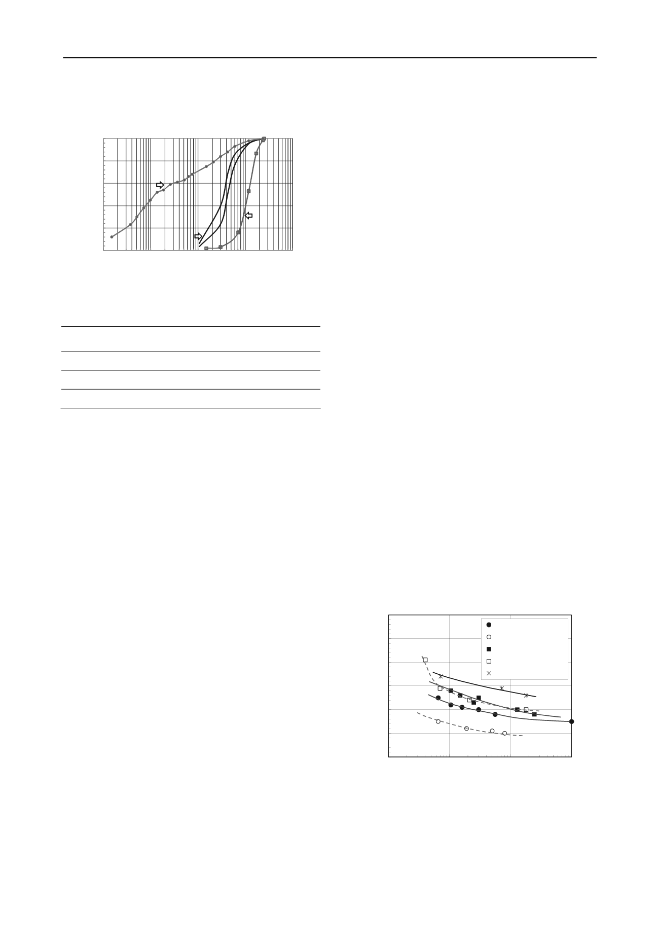
Figure 1. Grain size distribution curves of soils used in the tests.
3.2
Field tests
In this paper, the results of two sets of field tests are discussed:
cone penetration testing (CPT) and seismic dilatometer testing
(sDMT). These tests were performed near the two sites where
the undisturbed soil samples were obtained. The CPT was
performed every 100mm depth interval, while the sDMT was
carried out at every 500mm interval, with the first reading taken
at 1m depth from the ground surface. An electrically-operated
Autoseis hammer was used to generate a shear wave that
propagated through the ground. The shear wave signals were
recorded by the geophones in the seismic module and were sent
back to a computer system as seismographs for analysis
purposes. The seismographs from both geophones were shown
as similar waves but with the time lag due to the fact that one of
the geophones is 500 mm deeper than the other. A computer
program allowed the two seismographs to be re-phased and so
that the actual travel time difference of the shear wave could be
calculated. The shear wave velocity of the soil layer between
the two geophones was calculated from the interval between the
two geophones divided by the difference in travel time.
4 TEST RESULTS AND DISCUSSION
4.1
Effect of density on reconstituted pumice specimens
Orense et al. (2012) discussed the effects of relative density on
the liquefaction resistance of reconstituted pumice sands. The
curves for dense pumice specimen (
D
r
=70%), loose pumice
specimen (
D
r
=25%), as well as for the undisturbed Mikkelsen
Rd sample obtained (at 6.0-6.6m), corresponding to double
amplitude axial strain
DA
=5% are reproduced in Figure 2. The
slope of the curve for loose sand is gentle when compared to
that of dense sand, with the latter having higher cyclic
resistance. On the other hand, the slope of the curve for
undisturbed sample is as gentle as the loose reconstituted
samples, but the CSR (=
d
/2
c
’, where
d
is the deviator stress)
is about three times higher.
0
0.1
0.2
0.3
0.4
0.5
0.6
1
10
100
1000
Cyclic Shear Stress Ratio, CSR
Number of cycles, N
Pumice (Dr=25%)
Toyoura (Dr=50%)
Pumice (Dr=80%)
Toyoura (Dr=90%)
Undisturbed sample
Pumice (
D
r
=25%)
r
ice (
r
7
r
ndisturbed s le
Cyclic shear stress ratio,
d
/2
c
’
Nu ber of cycles,
N
Figure 2. Cyclic resistance curves for the samples used.
Also plotted in the figure are the cyclic resistance curves for
loose (
D
r
=50%) and dense (
D
r
=90%) Toyoura sand, as reported
by Yamamoto et al. (2009). Comparing the curves for Toyoura
sand and for reconstituted pumice sands, two things are clear:
(1) loose specimens have gentle cyclic resistance curves, while


