1569
Technical Committee 203 /
Comité technique 203
0
0.1
0.2
0.3
0.4
0.5
1
10
100
1000
Measured
Calculated
CSR
(a)
Sand 1
0
0.1
0.2
0.3
0.4
0.5
1
10
100
1000
Measured
Calculated
(b)
Sand 2
0
0.1
0.2
0.3
0.4
0.5
1
10
100
1000
Measured
Calculated
CSR
(c)
Sand 3
0
0.1
0.2
0.3
0.4
0.5
1
10
100
1000
Measured
Calculated
(d)
Sand 4
0
0.1
0.2
0.3
0.4
0.5
1
10
100
1000
Measured
Calculated
CSR
(e)
Sand 5
0
0.1
0.2
0.3
0.4
0.5
1
10
100
1000
Measured
Calculated
(f)
Sand 6
0
0.1
0.2
0.3
0.4
0.5
1
10
100
1000
Measured
Calculated
CSR
(g)
Sand 7
0
0.1
0.2
0.3
0.4
0.5
1
10
100
1000
Measured
Calculated
(h)
Sand 8
0
0.1
0.2
0.3
0.4
0.5
1
10
100
1000
Measured
Calculated
CSR
N
(i)
Sand 9
0
0.1
0.2
0.3
0.4
0.5
1
10
100
1000
Measured
Calculated
N
(j)
Sand 10
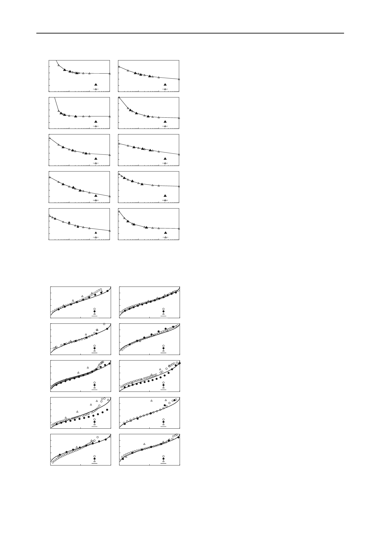
Figure 3. Comparison of measured and predicted
CSR – N
curves of soil
samples from Korea.
0
0.2
0.4
0.6
0.8
1
0
0.5
1
CSR= 0.30
CSR= 0.33
CSR= 0.35
β=1.2
Pore pressure ratio, r
u
(a) Sand 1
0
0.2
0.4
0.6
0.8
1
0
0.5
1
CSR= 0.25
CSR= 0.28
CSR= 0.30
β=1.1
(b)Sand 2
0
0.2
0.4
0.6
0.8
1
0
0.5
1
CSR= 0.20
CSR= 0.23
CSR= 0.25
β=1.0
Pore pressure ratio, r
u
(c) Sand 3
0
0.2
0.4
0.6
0.8
1
0
0.5
1
CSR= 0.20
CSR= 0.25
CSR= 0.30
β=1.4
(d)Sand 4
0
0.2
0.4
0.6
0.8
1
0
0.5
1
CSR= 0.20
CSR= 0.25
CSR= 0.30
β=1.1
Pore pressure ratio, r
u
(e) Sand 5
0
0.2
0.4
0.6
0.8
1
0
0.5
1
CSR= 0.25
CSR= 0.28
CSR= 0.30
β=0.7
(f) Sand 6
0
0.2
0.4
0.6
0.8
1
0
0.5
1
CSR= 0.20
CSR= 0.25
CSR= 0.30
β=0.7
Pore pressure ratio, r
u
(g)Sand 7
0
0.2
0.4
0.6
0.8
1
0
0.5
1
CSR= 0.30
CSR= 0.35
CSR= 0.40
β=0.9
(h)Sand 8
0
0.2
0.4
0.6
0.8
1
0
0.5
1
CSR= 0.22
CSR= 0.28
CSR= 0.33
β=1.4
Pore pressure ratio, r
u
Damage parameter, D
(i) Sand 9
0
0.2
0.4
0.6
0.8
1
0
0.5
1
CSR= 0.20
CSR= 0.25
CSR= 0.30
β=1.4
Damage parameter, D
(j) Sand 10
Figure 4. Comparison of measured and predicted pore pressure.
3 VALIDATION OF THE MODEL
The applicability of the model is evaluated through
comparisons with measured data set, the
CSR
–
N
curves of
which are displayed in Figure 3. The measurements and the
predicted pore pressures are compared in Figure 4.
D
ru
=1.0
is
calculated from
CSR
–
N
curves using Eq. (5).
were selected
by trial and error. The values of
are shown in listed in Figure
4. It was found that all pore pressure curves fall between the
upper bound (
= 1.4) and mean curve (
= 0.7). No curves
were shown to fall below the mean curve, consistent with
observations of Polito et al. (2008). Dependence of
on
SR
was
observed in three measurements (Sand 6, 7, 9), while other
measurements showed no or limited influence of
SR
. Even in
soils for which
SR
dependence is present, use of representative
value of
was shown to be acceptable.
If the pore pressure model is to be implemented in a time-
domain dynamic analysis program, the dependence of
SR
on
cannot be modeled since
SR
is not constant during a seismic
loading. The variation of
under transient loading is not yet
known. If it is expected that the soil will be largely influenced
by
SR
, it is recommended that the effective shear strain and
corresponding
SR
be calculated from uncoupled analysis, from
which the resulting
is selected and applied in the model
throughout the analysis.
4 METHOD FOR CONSTRUCTING EMPIRICAL
CSR – N
CURVE
The proposed pore pressure model cannot be used in the
absence of measured
CSR – N
curve. This section describes an
empirical method for constructing the
CSR – N
curve from in-
situ penetration test. This process is particularly useful since
field test measurements are always available.
The penetration resistance measured from a field test,
including the standard or cone penetration tests, are commonly
used to determine the cyclic resisting ratio (
CRR
) (Robertson
and Campanella 1985, Seed et al. 1983), which is defined as the
minimum
CSR
at which the liquefaction is triggered at the given
number of loading cycles. The empirical curves that relate field
measured penetration resistance (e.g. blow count from standard
penetration test or cone tip resistance from cone penetration
test) with
CRR
are typically developed for a magnitude (
M
) =
7.5 earthquake. It is a common practice to assign a value of 15
for the equivalent number of cycles for a
M
= 7.5 earthquake,
N
M=7.5
, based on the recommendation of Seed et al. (1975a). Liu
et al. (2001) have shown that the
N
M=7.5
ranges from 19 – 30,
depending on the magnitude, epicentral distance, near fault
directivity, and site effects. If the number of cycles for a
M
=
7.5 event is determined, the field test derived
CRR
and
N
M=7.5
data set can be used as a point of the
CSR – N
curve. The full
CSR – N
curve can be constructed by assigning
CRR
values
relative to the field test derived
CRR
value for a range of
N
values. The relative values of
CRR
can be calculated from the
normalized
CSR – N
curve, which is explained in detail in the
following.
Liu (2001) collected
CSR – N
curves from a large body of
literature and developed normalized
CSR – N
curve, where
CSR
was normalized by
CSR
N=15
, which represents the
CSR
at
N
=
15. The data showed that the shape of the normalized curve
depends on the relative density, method of sample preparation,
stress path (type of laboratory test), and compositional factors
such as gradation / angularity. It was concluded that the results
of simple shear tests performed at relative densities between 45
– 70%, using air/water-pluviated or moist-tamped soil samples
fall within a narrow band, as shown as dotted red lines in Figure
5. Also shown are the
CSR – N
curves from Figure 1 and Figure
2, but normalized to
CSR
N=15
. The curves of Liu (2001) are
close to the upper bound of the
CSR – N
curves calculated in
this study up to
N
= 15. It is consistent with the previous
findings that the cyclic triaxial tests result in flatter curve


