1197
Technical Committee 106 /
Comité technique 106
from ground surface and the depth of the wetting front. The
saturation front in t hours can be calculated from Eq. 1. The
wetting front can be determined by assuming by that it is equal
to the trapezoidal area and the accumulation amount of
infiltration. It is considered that the saturation front was 50 mm
because the pressure head will be 0 mm at the tensiometer
installed to a depth of 50 mm. The regression parameter of Eq. 1
can be estimated as follows:
s
r
s
f
H
D
Q
H
2
8
(2)
where are, A is the trapezoid area, is volumetric water content
of saturated soil and .
Q
is the amount of infiltration, and
D
is
the radius of cylinder.
4.2
Presumption of the moisture distribution using dynamic
state soil moisture distribution model
We performed a separate numerical simulation to verify
whether the moisture distribution had a trapezoid distribution.
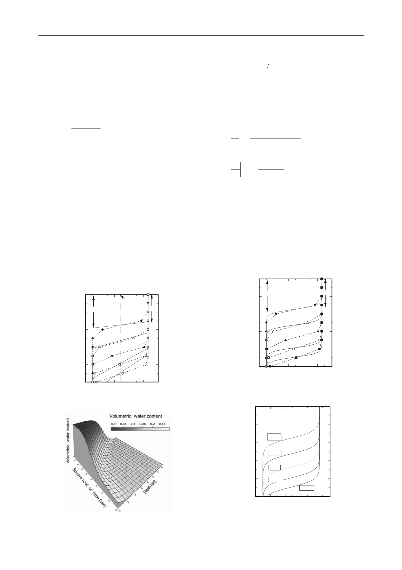
The result is shown in Fig. 7. In comparison with numerical
experimental results the inclines of the soil moisture distribution
that was approximated with a trapezoid increase and become
estranged. Moreover, the depth of the wetting front differed
from the result obtained in the numerical analysis.
On the other hand, the trapezoid distribution accords with the
numerical experimental result at the depth of the mean soil
moisture. The authors therefore selected the dynamic state
moisture distribution model to model moisture distribution
(Eq.3 and Fig. 8). In this model, parameter a, which indicates
the depth of the average moisture, and parameter b, which
0
1
2
3
4
5
0 0.1 0.2 0.3 0.4 0.5
Volumetric water contnet,
θ
Depth from ground surface,
z
(cm)
6sec
12sec
18sec
24sec
30sec
H
s
H
f
Dotted line
:
Simulation results
Solid line
:
Presumed results
θ
m
Figure 7. Inspection of the trapezoid distribution and water distribution
by the numerical value experiment.
Figure 8. Dynamic state soil moisture distribution model
indicates the slope of the moisture distribution, are required.
Since the average moisture can be inferred based on the initial
moisture
i
, is (
i
i
s
2
), the conditions of exp(0) =1 are
acquired. Therefore, if the depth zm is used as the average
moisture, then Eq.4 can be derived as follows:
i
m
i
s
bz a
exp 1
(3)
0
m
bz a
(4)
2
exp 1
exp
bz a
bz a b
z
i
s
(5)
4
b
z
i
s
z
m
(6)
where,
a
and
b
are parameters of the dynamical moisture
distribution model. Furthermore, the slope of the moisture
distribution differentiates an Eq.3 with respect to
z
, which can
be used to obtain Eq.5. Since Eq.5 is equivalent to the slope
(Eq.6) of the moisture distribution expressed using the depth of
a saturation front and
a
wetting front, parameter
b
can be
obtained.
Parameter
a
can be obtained using Eq.4 and the parameters of
an Eq.3 are identified. The result of the experimental and
numerical moisture distributions is shown in Fig. 9. The dashed
line shows the moisture distribution of the numerical
0
1
2
3
4
5
0 0.1 0.2 0.3 0.4 0.5
Volmetric water content,
θ
Depth from ground surface,
z
(cm)
6sec
12sec
18sec
24sec
30sec
H
s
H
f
Dotted line
:
Simulation results
Solid line
:
Presumed results
θ
m
Figure 9. Water distribution inferred numerically and using the
proposed method.
0
1
2
3
4
5
0 0.1 0.2 0.3 0.4 0.5
18sec
Volumetric water content,
θ
Depth from ground surface, z
(cm)
6sec
12sec
24sec
30sec
Figure 10. Presumed soil moisture distribution using the dynamic state
soil moisture distribution model.
experimental result, the solid line the estimated moisture
distribution from Eq.3. Fig. 9 shows that both are in agreement.
The experimental result in the permeation test (Fig.4) obtained


