1165
Technical Committee 106 /
Comité technique 106
point was 0.65 for Case 1 and 0.67 for Case 2. The saturation
degree of LNAPL was measured from the injection volume
when we observed the LNAPL in the plate at the outlet position.
Values were 80.1% for Case 1 and 83.1% for Case 2. These
similar values indicate that the prepared samples both had
similar pore structures at the initial condition.
3.2
KI solution injection into sand polluted by LNAPL
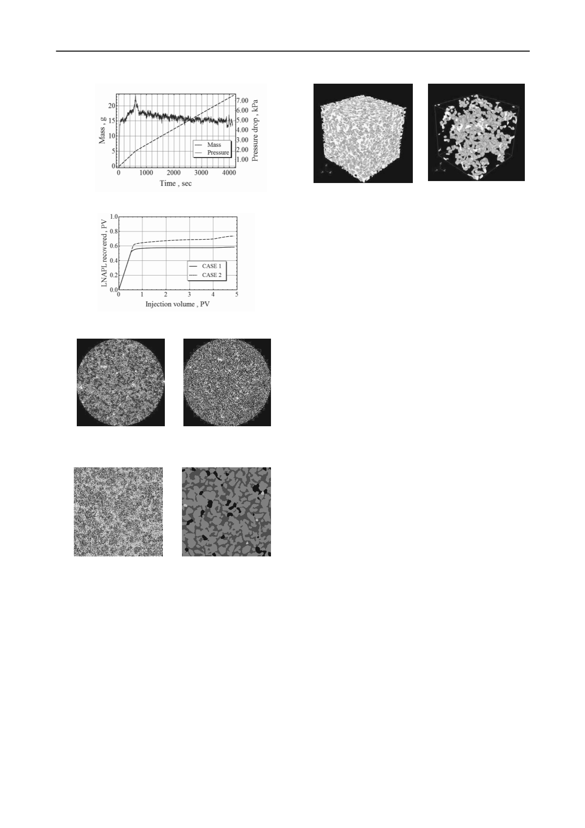
Figure 6 shows the volume profile of LNAPL recovered by KI
solution injection. As shown in Figure 6, the injection pore
volume at the breakthrough point was 0.51 for Case 1 and 0.56
for Case 2, indicating that the entry pressure for Case 1 was
observed earlier than Case 2. To evaluate this phenomenon, the
capillary number may help in the following equation (1):
Ca
= v
w
dal
w
/
where
v
dal
is Darcy’s velocity,
is kinematic viscosity, and
is
the interfacial tension. Subscript w
means “wetting.” The
capillary number
Ca
indicates the ratio of viscosity and
interfacial tension
,
and when
Ca
is less than 10
-6
multiphase
flow should be dominated by capillary pressure (Mayer &
Miller, 1993). In other words, a low
Ca
number may cause
fingering flow in porous media. In this study,
Ca
for Case 1 was
1.57 x 10
-6
and
Ca
for Case 2 was 3.14 x 10
-5
. LNAPL
saturation degrees after the KI solution injection test in Case 1
and Case 2 were 21.5% and 9.5%, respectively, confirming that
Ca
greater than 10
-6
caused less volume of residual LNAPL.
3.3
Evaluation of pore structure using the MCW method
Figure 7 shows MXCT images of sand after injecting LNAPL
(Figure 7(a)) and KI solution (Figure 7(b)) in Case 1. X-ray CT
images are generally 256-level grayscale, with black areas
having the least density and white areas the greatest. Figure 7(a)
shows that LNAPL was trapped, and its shape was different.
Also, the black shape of LNAPL in Figure 7(b) was more
circular than as seen in Fig 7(a). These LNAPL blobs are
residual LNAPL trapped due to KI solution injecting. Multi-
threshold processing with the MCW method was applied to a
CT image with 512 × 512 × 512 cubic voxel area. The 4-color
MXCT image shown in Figure 8(b) was created from Figure
8(a).
Based on 4-color CT images, only pore structure and residual
LNAPL could be extracted from the CT images in Figure 8(b).
The porosity obtained from 3D CT images was 40.7% for Case
1 and 38.5% for Case 2. In fact, the porosity calculated from the
mean dry density of the sand sample was 39.4%, and the
difference should be negligible (<1% error), confirming that
multi-threshold processing with MCW gave reasonable values
for porosity. Residual LNAPL after injecting the KI solution
was 16.7% for Case 1 and 12.6% for Case 2. Measured
saturation of residual LNAPL from the mass in the outlet plate
was 4.8% less than the obtained value from MCW for Case 1,
and 3.1 % greater than that for Case 2.
Figures 9(a) and 9(b) show 3D CT images of pore structure
and LNAPL blobs isolated with MCW processing. Pore
structure and LNAPL blobs were thus successfully extracted
from soil samples in three dimensions without disturbance.
3.4
Cluster analysis of pore structure
Figures 10 shows histograms of pore size in Case 1 and Case 2.
Frequency in vertical axis means the normalized value by total
voxel number of pore structure. Maximum pore size in Case 2
was slightly greater than in Case 1, as shown in Figure 10.
There were 1317 pore elements with LNAPL in Case 1 and
1023 in Case 2. Table 3 summarizes saturation degrees of
LNAPL for Case1 and Case 2 before and after KI solution
injecting obtained from X-ray CT images treating MCW
processing. Initially, the sand sample for Case2 had only 3%
greater saturation degree of LNAPL than Case 1. However,
residual saturation degree of LNAPL for Case 2 was less than
(a)
LNAPL injecti
on under KI
saturation conditions
(b) KI solution
injection after
the status of Fig. 7(a)
(
b) Partial MXCT image
after MCW processing
(
a) Partial MXCT image
before MCW processing
Figure 6. Volume profile of LNAPL recovered in Cases 1
and Case 2
Figure 7. MXCT images after injecting LNAPL and KI
solution
(a) Pore structure
(b) Residual LNAPL distribution
Figure 5. Pressure difference between inlet and outlet
and cumulative fluid mass in Case 1
Figure 8. MXCT images after MCW processing
Figure 9. MXCT images after MCW processing


