1164
Proceedings of the 18
th
International Conference on Soil Mechanics and Geotechnical Engineering, Paris 2013
isoparaffin, which has a fluid density of 0.75 g/cm
3
. Figure 2
shows the MXCT experimental setup, and Table 2 shows the
scanning conditions.
2 IMAGE PROCESSING ANALYSIS
2.1
Marker-controlled watershed processing
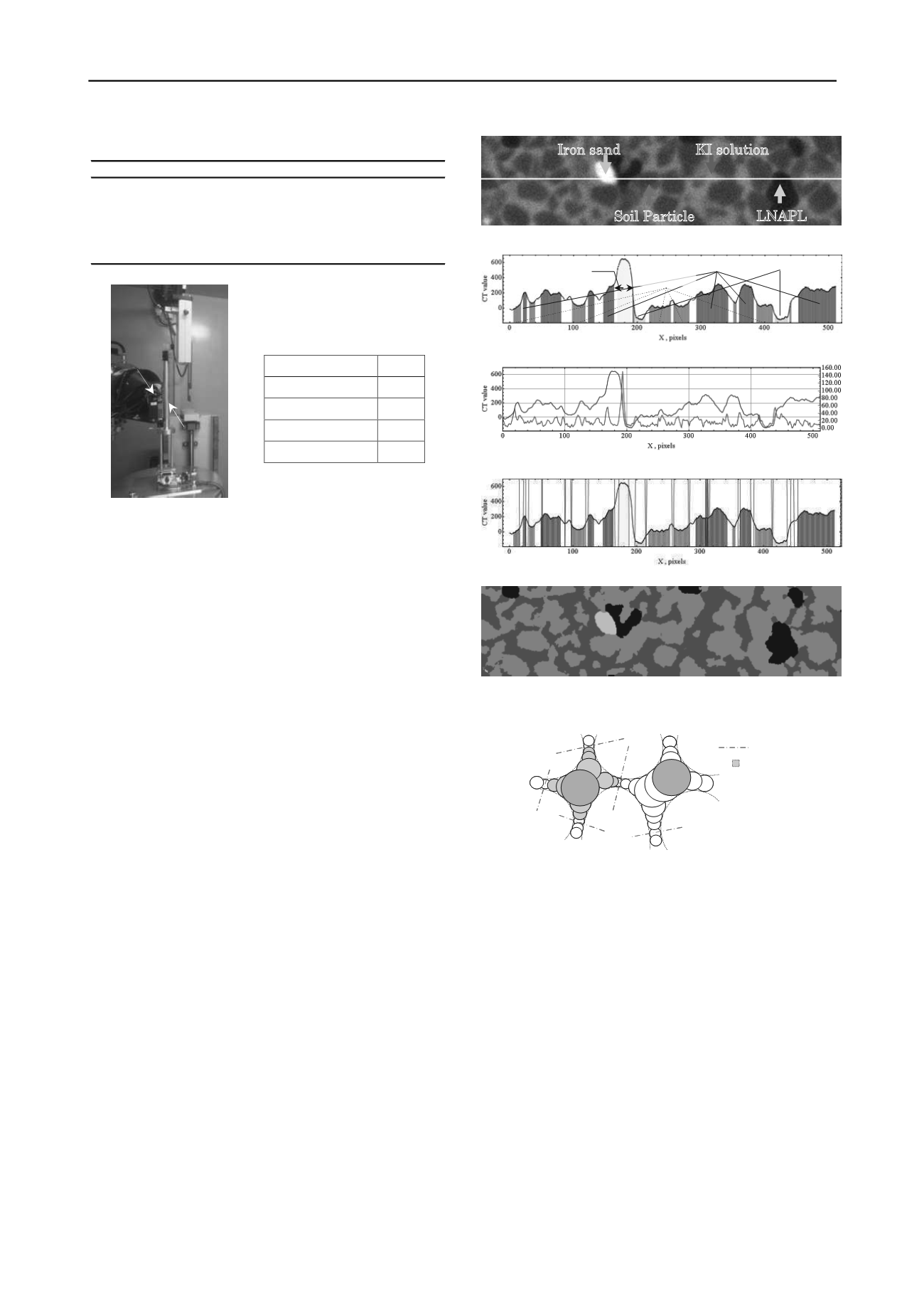
X-ray CT images are composed of voxels, called CT-values,
which are proportional to the material density. To separate pore
space and soil particles in the image, it is necessary to define a
threshold value for the CT values. Figure 3 shows an X-ray CT
image of Toyoura sand that includes KI solution and LNAPL.
That image also includes magnetic sand, so four kinds of CT-
value exist in the CT image of Figure 3(a): soil particles, solid-
phase magnetic sand particles, KI solution, and liquid-phase
LNAPL. Knowing the number of materials in the CT images
allows fixing areas of magnetic sand particles, soil particles,
LNAPL, and pore space, as well as identifying mixels where
two or more materials occupied a single voxel. Watershed
processing, which is based on CT-value gradient changes
between materials, was applied only to mixel areas in what is
called the marker-controlled watershed (MCW) method. Figures
3(b)
–
(d) show the MCW process. Figure 3(b) is the CT-value
profile obtained from lines in the CT image in Figure 3(a).
Clarification of the materials in the CT image allows defining
the CT-value range for each material without knowing CT-
values for the mixel. To evaluate the gradient in the mixel areas,
Figure 3(c) shows a profile of the gradient obtained from Figure
3(b). Finally, the coordinate in the CT image with maximum
gradient was defined between different materials, and watershed
processing was applied to the CT image. This CT-value
thresholding technique does not lose spatial geometry
information, and is an objective approach for distinguishing the
CT threshold values.
2.2
Image analysis technique for connectivity of pore
structure based on mathematical morphology
Mukunoki et al. (2011) proposed an image processing technique
that uses mathematical morphology (Soille, 2002) to evaluate
the 3-D distribution of pore scale in dry, sandy soil (a two-phase
soil particle and air mixture). We used this method to evaluate
the volume and diameter of pore water, and showed that
LNAPL existed in pore structures. Moreover, connectivity of
the pore structure affects flow behavior, and so should be
considered in this study. If continuous structures could be
isolated as part of a pore structure, a cluster labeling method
would give the number of isolated LNAPL blobs and their
connectivity. The authors applied the evaluation method of the
3D distribution of pore scale, and used this method to find a
circle with minimum diameter as shown in Figure 4. This
method successfully separated entire pore structures, making it
possible to evaluate spatial distribution of the LNAPL volume
.
3 RESULTS AND DISCUSSION
3.1
LNAPL injection to the sand with saturation of 100%
Intrinsic permeability (k) of the tested sand was 1.75 × 10
-11
m
2
for Case 1 and 1.57 × 10
-11
m
2
for Case 2, as obtained from the
injection test. In this study, the injection speed was a parameter
for this test. Figure 5 shows the difference between inlet and
outlet pressures, and the mass of fluid collected at the outlet for
Case 1. The injection pore volume (PV) at the break-through
Core
Core
Watershed
element
Iron sand
Soil Particle
LNAPL
KI solution
KI solution LNAPL
Iron sand
Soil
(a) Partial CT image
(b) Selection of marked area in the CT-value profile
(c) Extraction of gradient in the CT-value profile
(d) Definition of marked areas in the CT-value profile
(
e) X-ray CT image treated with MCW processing
Table 2. Scan conditions
Voltage (kV)
180
Current (μA)
200
Number of view angles
1500
Projection average
10
Resolution (μm)
5
Property
LNAPL KI solution
density
ρ
(g/cm
3
)
0.7486
1.24786
viscosity
ν
(cP)
1.29
0.9664
Surface tension
γ
(dyn/cm)
20.0
72.3
contact angle
• •
(degree)
6.4
62.1
interfacial tension
γ
nw
(dyn/cm)
54.5
MOLD-STORE SAMPLE
X-RAY TUBE
Figure 3. Marker-controlled watershed processing
Figure 4. Schematic of analysis method
Table 1. Specification of fluids tested
Figure 2. A photograph
of scene before CT
scanning


