1860
Proceedings of the 18t
h
International Conference on Soil Mechanics and Geotechnical Engineering, Paris 2013
centre. In other words, a node is covered if at least one facility
is located within the maximal service distance of that node.
Otherwise, the node is uncovered. If a network operator
instinctively places all the available resources on the nodes with
the greatest nodal weight (e.g. population), the outcome will not
necessarily be maximum coverage of the population by the
public facilities because of the likely overlaps and gaps in the
coverage of the demand nodes.
In reality, the 100% coverage target is not always achievable
due to limitations in the availability of supply units. If the
resources are insufficient to cover all the demand nodes, the
objective changes to cover as many nodes as possible within
S
using the limited resources. Figure 1 represents a typical
discretized network of demand nodes which could be
considered as the potential locations for accommodating the
additional facilities. With a sufficiently large maximal service
distance, for example, a single facility can cover all the demand
nodes on the network; hence
S
is a key decision parameter.
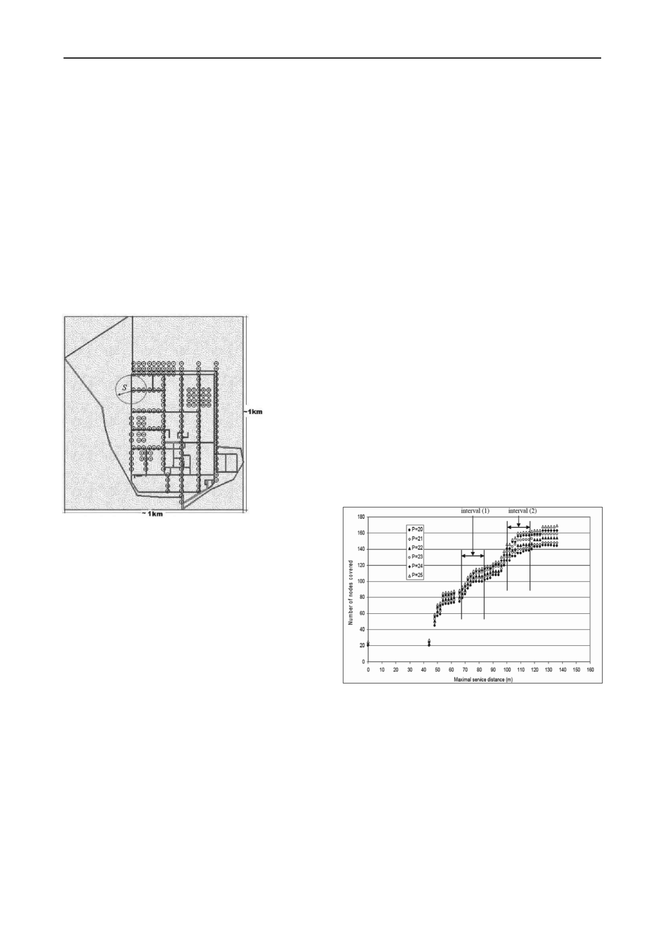
Figure 1. The concept of maximal service distance.
The MCLP is expressed as: Maximize coverage (population
covered) within a desired service distance by locating a fixed
number of facilities (Church and ReVelle, 1974).
The mathematical formulation of the MCLP in the context of
augmentation of a groundwater monitoring network is presented
in Hudak & Loaiciga (1992). Groundwater monitoring network
augmentation incorporates the following stages:
Discretize the model domain into a network of potential
detection monitoring sites (nodes).
Assign weighting to each node to quantify its relative
importance for coverage by a monitoring well.
Solve MCLP with successive values of
S
until target areal
plume coverage is achieved.
Determine the corresponding configuration of the added
wells on the network.
2.1 Geometry of the grid (problem domain discretization)
An irregular grid of 188 nodes was defined within the oil
refinery area taking into account the local hydrogeology as
compared to similar cases where groundwater monitoring
networks has been augmented, the limitations against
excavation of wells on site, the spacing between the existing
wells and the computational limitations for a plausible nodal
weight estimation. Each of the 15 existing wells was assigned to
the nearest node.
2.2 Nodal weight estimation
Due to the complex hydrogeological setting of the site and
presence of a large number of potential sources of oil
contamination within the refinery, using physical / numerical
models to calculate the nodal concentrations (weights) was
considered impractical. Kriging as a stochastic interpolator was
employed instead to estimate the weights. The groundwater
chemical data obtained from all 22 available monitoring wells
located within and around the refinery were utilised in this
nodal weight estimation.
2.3 Results
The budget allocated for additional monitoring wells included
the addition of a maximum 10 number to the existing network.
Therefore, the MCLP model was solved for different values of
P
from 20 to 25, noting
P
is the total number of existing and
additional wells on the network and there were 15 existing
wells. There were three key decision parameters; areal plume
coverage which corresponds to the vertical axis on Figure 2 and
is defined as the percentage of the nodes with weight values
above zero covered by one or more wells (i.e. located within
distance
S
of one or more wells), the total number of existing
and added wells (
P
), and the maximal service distance
S
(horizontal axis on Figure 2). The marked increase in the slope
of the curves on Figure 2 in two particular regions demonstrated
that with a moderate increase in the value of
S
, the areal plume
coverage would increase considerably compared to the other
regions on the curves. If the values of
S
and the number of
covered nodes (i.e. areal plume coverage) within these regions
(intervals) were reasonable for decision making, then it would
be possible to focus on these two regions for taking the next
steps towards the final decision. The maximal service distance
(
S)
plays the most important role in dictating the final
configuration of the added facilities. This parameter should
ideally be calculated through field, laboratory and theoretical
investigations. Considering the grid size of the study area,
values of
S
in the order of 100m were justified in this study.
Figure 2. The coverage trend curves.
Figure 3 demonstrates that within the maximal service
distance of 76m, it was possible to achieve a maximum areal
plume coverage of 60% (i.e. 113 covered nodes out of total 188
nodes could be covered). This amount of coverage was not
considered satisfactory. Therefore, the first interval on Figure 2
was not considered further and the second interval was selected.
Figure 4 illustrates the variation of maximal service distance
S
versus
P'
(number of monitoring stations to be added). Points
with unjustified values of
S
were not depicted on the graph.
Figure 4 demonstrated that augmenting the network with 10
additional monitoring wells was somewhat insensitive to the
magnitude of
S
, i.e. selection of 10 additional monitoring
stations would result in a considerable increase in the areal
plume coverage with minimum change in
S
. Hence, the network
was augmented with 10 additional boreholes, corresponding to
the areal plume coverage of 85% and
S
~108 m. The pattern of
additional wells showed no clustering at the areas of high


