716
Proceedings of the 18
th
International Conference on Soil Mechanics and Geotechnical Engineering, Paris 2013
and
y
directions, respectively. Energy slopes
S
fx
and
S
fy
can be
estimated by using the Manning formula as follows:
3/4
2
2
2
h
v uun S
fx
,
3/4
2
2
2
h
v uvn S
fy
(3)
where
n
denotes the Manning’s roughness coefficient. The
above shallow water equations are obtained by integrating the
Navier
–
Stokes equations over the flow depth with the
assumptions of the uniform velocity distribution in the vertical
direction and the hydrostatic pressure distribution. Although the
overflowing water of an embankment does not maintain the
hydrostatic pressure distribution when it undergoes rapid
changes in the bed slope on the crest, equation (1) is adopted as
the governing equation for the water flow onto the
embankments for simplicity.
The progression of soil erosion, induced by overland flows,
can be described as follows:
1
E
t
z
(4)
where
E
and
denote the erosion rate and the porosity of the
soil bed, which means the embankment surface here,
respectively. The erosion rates of soils are related to the bed
shear stress, and previous studies on this topic have found the
following relationship between the erosion rates and the bed
shear stress:
c
c
c
E
0
)
(
(5)
where
and
are the material constants for the erodibility of
soils and
c
denotes the critical bed shear stress which
determines the onset of bed erosion. Bed shear stress
is
obtained from energy slopes
S
fx
and
S
fy
as follows:
2
2
fy
fx
f
S S gh
S
(6)
where
is the density of water. In this analysis, the governing
equations are the system of the partial differential equations of
equations (1) and (4), and the four variables to be solved are
h
,
u
,
v
and
z
.
3 NUMERICAL METHOD
3.1
Finite volume method
So far, several numerical methods have been proposed to solve
the shallow water equations. We employ the basic procedure
proposed by Yoon & Kang (2004) and apply the concept of the
surface gradient method (SGM) by Zhou et al. (2001) to the
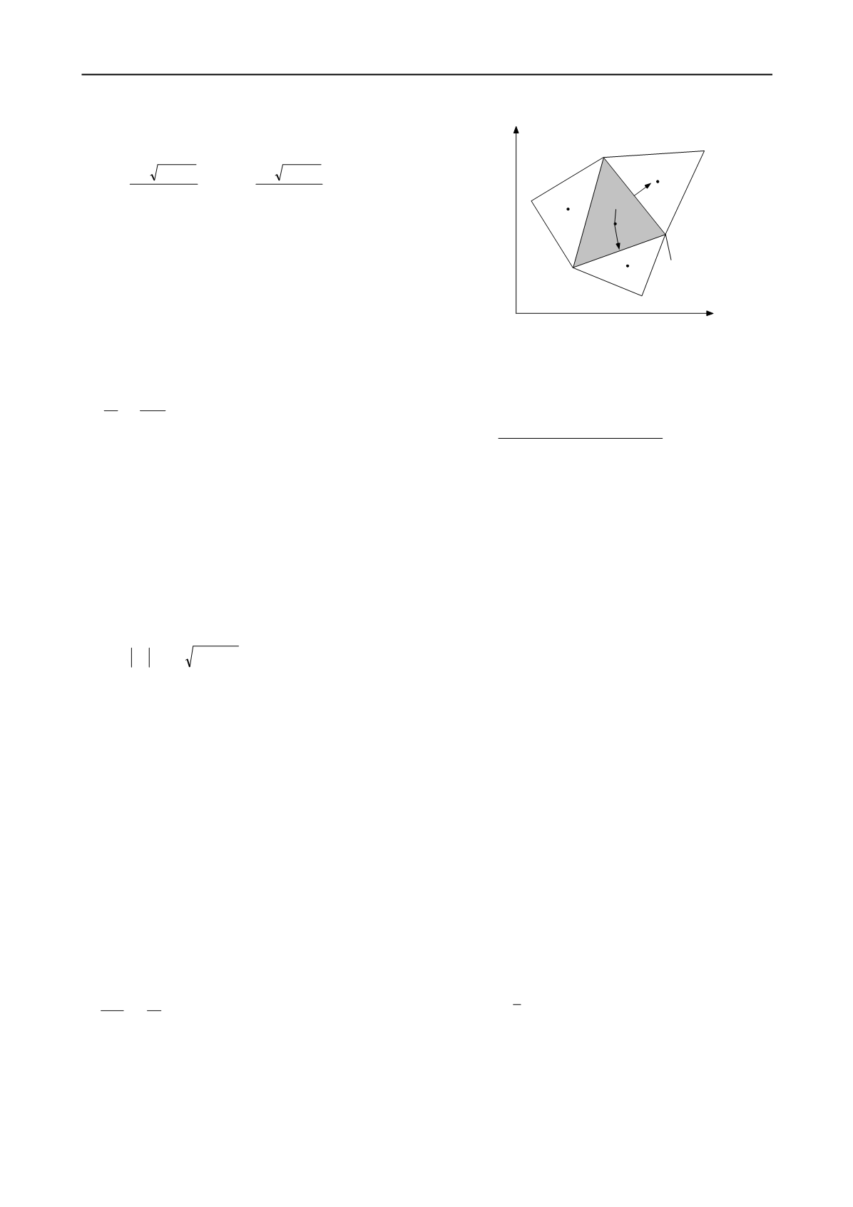
reconstruction of the state variables. A finite volume approach
to unstructured grids is applied to equation (1) and the
triangular cells are used for the spatial discretization. As shown
in Figure 1, state variables
u
,
v
and
h
are stored at their
centroids, while variable
z
is computed at the vertices of the
triangular cells. Integrating equation (1) over the area of the
i
th
triangular cell, the following spatially discretized equations are
derived with the aid of the divergence theorem:
i
j
ij
ij
i
i
A dt
d
S
E
U
3
1
*
1
(7)
where
U
i
,
S
i
and
A
i
denote the state vector, the source term
vector and the area of the
i
th cell, respectively,
E
*
ij
is the normal
flux through the
j
th side of the cell, and
ij
is the length of the
side. Normal flux
E
*
ij
is computed at the cell face by a Riemann
L
k
j=
1
j=
2
j=
3
x
y
t
=(
t
x
, t
y
)
o
z
k
U
i
i
R
r
ij
Figure 1. Triangular cells and placement of variables.
solver. This study employs the approximate HLL Riemann
solver proposed by Harten et al. (1983), which determines the
normal intercell flux as follows:
0
0
0
)
(
*
R
R
L
L
R
L
R
L
R R L
R L
L R
L
S
S
S
S
S S
SS
S
S
E
U U
E E
E
E
(8)
where subscripts L and R mean the left and the right sides of the
cell boundary. (The direction of the outward normal vector is
considered rightward.) The values with subscripts are defined at
the middle of the cell sides and are calculated by the linearly
reconstructed data explained later.
S
L
and
S
R
are the wave
speeds. The detailed procedures for computing the wave speeds
and the normal flux are referred to in Yoon & Kang (2004).
3.2
Linear reconstruction and surface gradient method
To achieve second-order-accuracy of the numerical computation,
the variables, such as
u
and
v
, need to be linearly distributed
within the finite volume cells, each of which stores their values
at the centroids. This procedure is carried out based on the data
of the neighbouring cells and is called linear reconstruction.
When a variable
is linearly reconstructed on the
i
th cell, the
following procedures are to be completed:
1. The unlimited gradient
of the cell, which means the
regular or the ordinary gradient, is evaluated using the data
at the centroids of the neighbouring cells.
2. The limited gradient
l
of the cell is calculated from the
unlimited gradients of the cells shearing the interfaces.
3. The following linear interpolation with the obtained limited
gradient reconstructs the variable on the cell:
l
i
i
i
i
rec
i
) (
) (
r
r
(9)
where
r
i
is the position vector relative to the centroid of the
i
th cell and
) (
i
rec
i
r
is the reconstructed variable on the cell
as a function of
r
i
.
Details of the above first and second procedures, for calculating
the unlimited and the limited gradients, are referred to in Yoon
& Kang (2004).
The state variables of the shallow water equation,
u
,
v
and
h
,
must be evaluated at the cell interface in order to compute the
normal flux given by equation (8). Let the height of water
surface
h+z
) at the
i
th cell centre be defined as
k
k
i
i
z
h
3
1
(10)
where subscript
k
is the index for the cell vertices. (Note that the
values of
z
are not stored at the centroids, but at the vertices.)
The surface gradient method (Zhou et al. 2001), which
guarantees stable computation of steady solutions, gives the
state variables at the midpoint of the
j
th side, (
uh
)
ij
, (
vh
)
ij
and
h
ij
,
as follows:
l
i
ij
i
ij
uh
uh
uh
)
(
) ( ) (
r
(11)


