1293
Technical Committee 202 /
Comité technique 202
Table 1. Material parameters used in analyses
Notes:
Poisson’s ratio considered 0.3
From 1D consolidation tests
* At top of soil layer
‡
Gradient of
0
c
p
after -14.5 m 5.5 kPa/m of depth
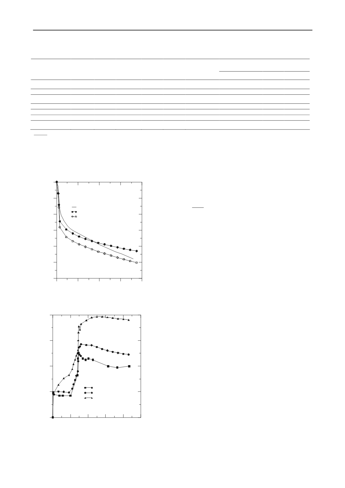
The excess pore water pressure was monitored for 217 days and
observed to be better predicted by the MCC than EVP model.
Up to 73 days, the MCC model captured the measured excess
pore water pressure well but then started to over-predict it.
Figure 4. Comparison of measured and predicted settlements
Figure 5. Comparison of measured and predicted excess pore water
pressures
4 OBSERVATIONAL APPROACH
Observational approaches, such as the Asaoka (1978) and
Hyperbolic (Tan 1995) methods, allow predictions of the
ultimate settlement of estuarine clay. In Asaoka (1978) method,
settlement (
t
) at any time (
t
) can be expressed as a linear plot
defined by Eqn. 1 and the ultimate settlement by Eqn 2.
0 1 1
t
t
(1)
0
1
1
ult
(2)
where
0
1
,
are the co-efficients representing the intercept and
slope of the fitted straight line proposed by Asaoka (1978)
respectively, and the intercept point of the fitted line and 45
lines stands for the ultimate settlement. Applicability of Asaoka
method for predicting the creep-included settlement of soft
clays has been questioned previously (Islam et al. 2012,
Lansivaara 2003). Moreover, effectiveness of the Asaoka
method is biased by the selection of the time interval (
t
). For
these reasons, in the present study, the prediction of the ultimate
settlement obtained from the Asaoka method was compared
with the ultimate settlement prediction from ‘Hyperbolic’
method.
For Asaoka Plot, the settlement data obtained for the
settlement plate (SP18) was extracted for a particular constant
time interval value
t
(e.g. 7 days) and the maximum
monitored settlement over the field monitoring period was
considered as the peak settlement value. By trial and error,
consideration of the settlement-time data range after 60%
consolidation was found to be appropriate for predicting the
ultimate settlement of the NBR embankment using Asaoka
method. Similar approaches have been reported by Tan (1996)
which was supported by Bergado et al. (1991).
Different values of
t
( = 7, 14 and 21 days) were attempted
for predicting
ult
. It was observed from the application of
Asaoka method for this field case that, with increases in the
time interval (
t
), the predicted ultimate settlement decreased
but, after a certain cutoff time interval (
t
), their magnitudes
became identical which is in agreement with the findings of
Arulrajah (2005). The regression value for the corresponding
Asaoka plot was found to be about 0.99.
For the NBR embankment, the ultimate settlement
predicted using the Asaoka and Hyperbolic methods were
almost identical (517.00 mm and 517.25 mm respectively). In
both cases, data beyond 60% of the consolidation (Tan 1996)
were considered, as supported by Bergado et al. (1991). It is
therefore concluded that when the soft soil exhibits significant
creep, the ultimate settlement prediction by the Asaoka method
only provided good agreement with the Hyperbolic method after
a certain cutoff time interval (
t
) and the data range after 60 %
consolidation state. Therefore, the ultimate settlement prediction
by the Asaoka method for creep-susceptible soft estuarine clay
requires scrutiny.
Vertical permeability coefficients
RL (m)
M
N
e
0
K
0
c
p
*
(kPa)
i
K
(m/day)
0
e
k
C
Fill Materials
---
---
---
---
0.42
E
3000 kPa,
=35
,
c
= 5.0 kPa
+1.5 to -0.5
1.51
0.43
0.043
4.10
0.40
50.00
2.50×10
-5
1.70
1.00
-0.5 to -2.5
---
---
---
---
0.50
E
5000 kPa,
= 32
,
c
= 4.0 kPa
-2.5 to -9.5
1.33
0.39
0.062
3.85
0.46
80.00
2.5×10
-5
1.70
1.00
-9.5 to -14.5
1.20
0.23
0.030
2.70
0.50
112.00
2.5×10
-5
1.70
1.00
-14.5 to -19.5
1.07
0.13
0.013
2.51
0.55
114.00
‡
2.5×10
-5
1.70
1.00
-19.5 to -32.5
---
---
---
---
0.42
E
15000 kPa,
= 35
,
c
= 50.0 kPa
0
100
200
300
400
Time (Days)
-600
-500
-400
-300
-200
-100
0
Settlement (mm)
Measured
MCC
EVP
0
50
100
150
200
250
Days
0
20
40
60
80
Excess Pore Water Pressure (kPa)
PP1
MCC
EVP


