3522
Proceedings of the 18
th
International Conference on Soil Mechanics and Geotechnical Engineering, Paris 2013
2008) and FHWA (Berg et al., 2009) recommended
!
be
approximated to the site corrected PGA for walls less than
approximately 6 meters. Few publications can be found that
contain detailed discussions on this issue. Therefore, this paper
will present an approach for estimating seismic earth pressures
acting on rigid walls by considering more general base and wall
conditions and to provide a more detailed discussion with
respect to the relationship between
!
and PGA by considering
the momentum equivalent. Simplified seismic earth pressure
equations directly related to PGA are proposed for use by
engineers in their daily practice.
2
PSEUDOSTATIC NUMERICAL SIMULATION
Although response analysis is a good method for the evaluations
of seismic earth pressures, it is usually complicated and not
suitable for routine practice. In this study, pseudostatic
numerical simulations were initially performed for various
conditions. Simplified equations were then derived based on the
numerical simulation results.
2.1
Finite element method (FEM) modeling
Three cases were considered, 1) a restrained rigid wall and its
retained soils supported by a rigid base, 2) a restrained rigid
wall and its retained soils supported by a non-rigid base, and 3)
a rigid wall and its retained soils supported by a non-rigid base,
where a
restrained rigid wall
refers to a wall without horizontal
as well as rotational movement and a
rigid wall
refers to a wall
restricted in rotational movement only. Comparing the scale of
the wall and its retained soil mass, the mass mobilized by an
earthquake is much larger and the area of movement is much
broader. As such, Case 3 is considered to be more
representative to real situation.
The finite element models for the three cases are shown in
Figure 1. In Cases 1 and 2, the wall was completely fixed both
in the
x
-direction and rotation. In Case 3, the wall was only
fixed for rotational movement and was allowed to move
horizontally together with the deformation of the base at the
bottom of the wall. To delimit the boundary effects, a model
width was taken as 5 times the wall height. Furthermore, the
right-side boundary was switched from fixed in the
x
-direction
under gravity load to free in
x
-direction when inertial force was
applied. Details are shown in Figure 1.
a) Restrained rigid wall on rigid base
b) Restrained rigid wall on non-rigid base
c) Rigid wall on non-rigid base
Figure 1. Finite element modeling
Soil retained by the wall was assumed to be elasto-plastic
material and modeled using Mohr-Coulomb failure criteria. The
initial modulus of elasticity of this layer was chosen such that it
represents a dense sand material. Internal frictional angles
varying from 30 to 38 degrees were analyzed to confirm the
effect of strength parameters. To model the non-rigid base, a
layer of material with a modulus of elasticity corresponding to
soft bedrock material was utilized below the wall and its
retained soils. The depth of this layer was taken as equal to the
height of the wall. To shorten the calculation time, the material
comprising this layer was assumed to be linear elastic.
After finishing the FEM modeling, the calculations were
performed in steps. The stress field under gravity force was
calculated in the first step. Inertial forces were then applied by
adding horizontal seismic coefficients in the subsequent steps.
The right-side boundary was switched from fixed in the
x
-
direction and free in the
y
-direction to free in the
x
-direction and
fixed in the
y
-direction so that no tension would be created in
the soils near the right-side boundary.
A commercial finite element analysis program, Strand7, was
utilized in the analysis.
2.2
Earth pressures under pseudostatic load
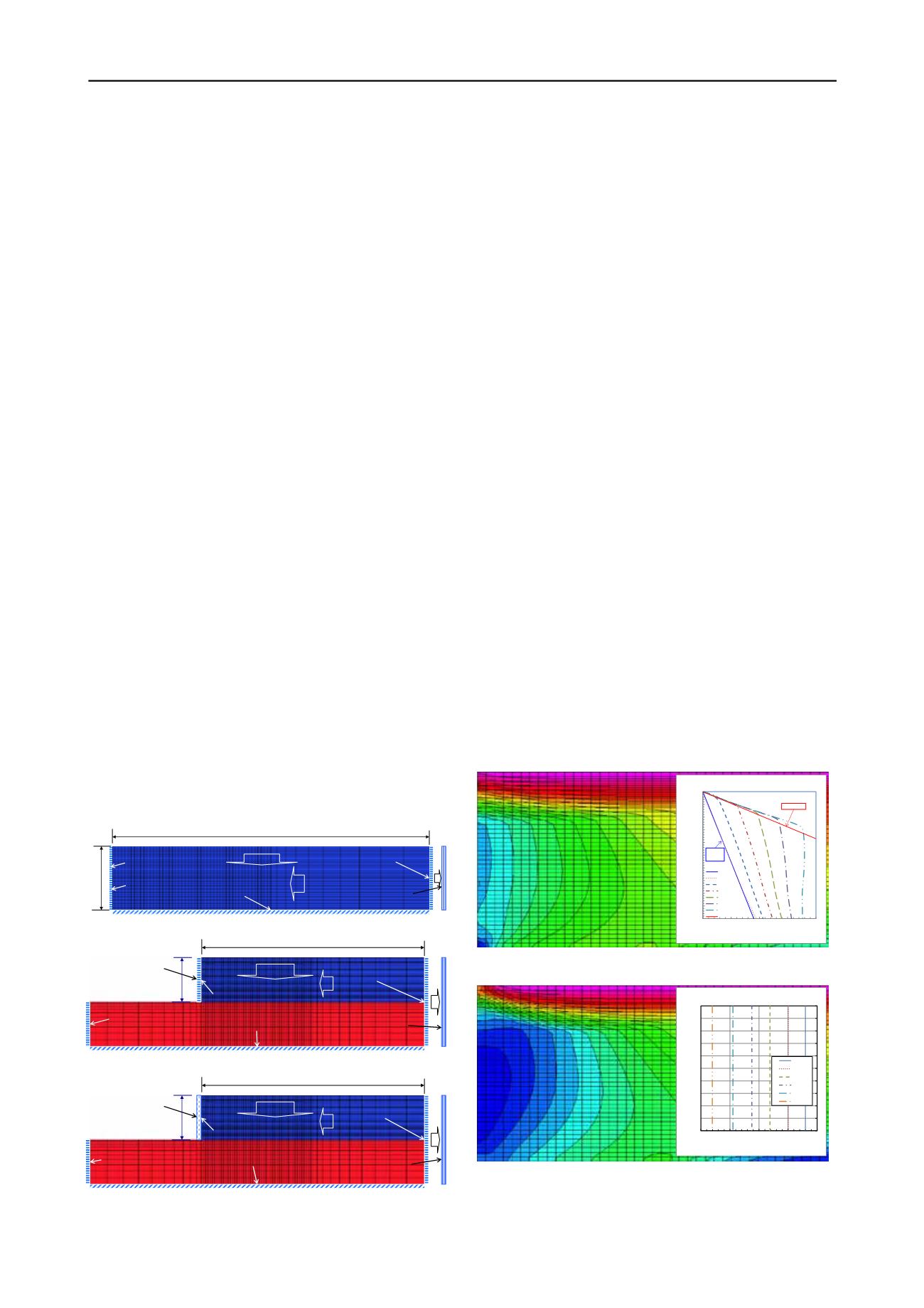
The typical horizontal stress distributions for a seismic
coefficient of
!
= 0.5
in the retained soil mass behind the wall
are shown as color contours in Figure 2 for a) a restrained rigid
wall on non-rigid base and b) a rigid wall on non-rigid base,
respectively. Figure 2 a) also shows the horizontal stress, or
earth pressure, distribution behind the wall for a seismic
coefficient that varied from 0 to 0.5. It can be seen that the
calculated stress distribution under
!
= 0.0
(gravity only) is
consistent with at-rest earth pressure calculated by the equation,
(1 − )
. It was also noticed that the distributions of
seismic earth pressures fall into a zone which is defined with the
at-rest earth pressure as the lower boundary and with the
passive earth pressure as the upper boundary. Theoretically, this
is true. Considering the relative movement, an applied inertial
force should be equivalent to passive wall movement. As such,
an increase in inertial force will eventually result in a passive-
type failure within the soil mass.
a) Distribution of horizontal stresses in retained soil mass at
!
= 0.5
and pressure distributions on the wall for various
!
b) Distribution of horizontal stresses in retained soil mass at
!
= 0.5
and wall movement for various
Figure 2. Typical results of pseudostatic finite element analysis, a)
restrained rigid wall on non-rigid base; b) rigid wall on non-rigid base
H
5H
Gravity
k
H
Fixed in X
& Rotation
Fixed in X
Changed to
Fixed in Y
Fixed in XY
Wall
5H
H
Fixed in X
Fixed in X
Changed to
Fixed in Y
Fixed in XY
Fixed in X
& rotation
Gravity
k
H
Wall
5H
H
Gravity
k
H
Fixed in X
Fixed in X
Changed to
Fixed in Y
Fixed in XY
Fixed in
rotation
Wall
0
0.1
0.2
0.3
0.4
0.5
0.6
0.7
0.8
0.9
1
0
1000
2000
3000
4000
z/H
HorizontalStress,σ
x
Non-‐RigidBase,RestrainedRigidWall
P0
kh=0.0
kh=0.1
kh=0.2
kh=0.3
kh=0.4
kh=0.5
Pp
At-‐rest
P
0
PassiveP
p
0
0.1
0.2
0.3
0.4
0.5
0.6
0.7
0.8
0.9
1
-‐0.0002 -‐0.00015 -‐0.0001 -‐0.00005
0
z/H
HorizontalDeformation
WallMovement
Gravity
kH=.10
kH=.20
kH=.30
kH=.40
kH=.50


