2178
Proceedings of the 18
th
International Conference on Soil Mechanics and Geotechnical Engineering, Paris 2013
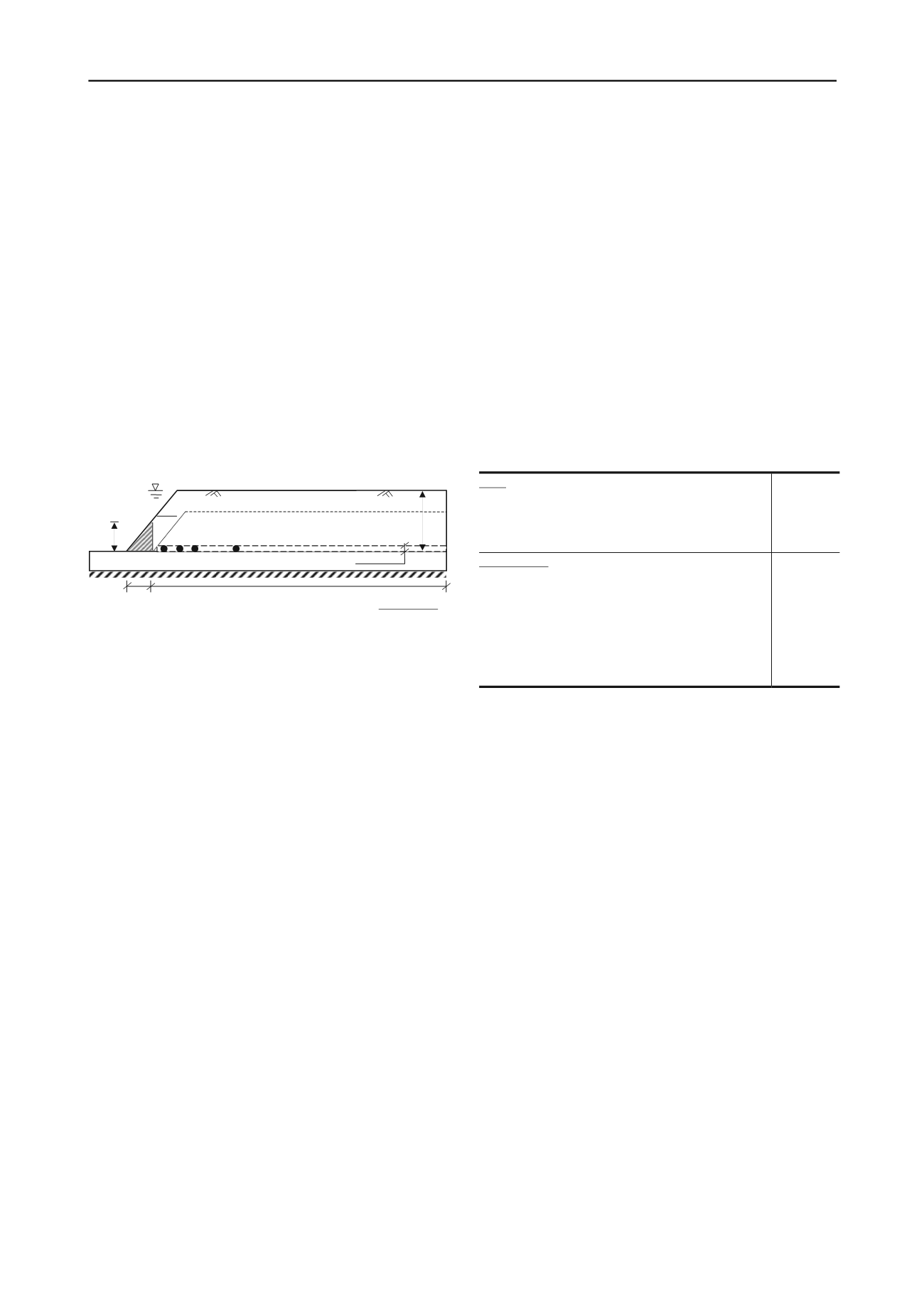
groundwater table is assumed at the crest of the slope and the
river is full. A block of soil near the toe of the slope shown by
the hatched zone is removed, which could be caused by erosion
or by excavation in the field. This block will be referred as
“excavated/eroded soil block.” It is also assumed that the
erosion or excavation is occurred relatively fast such that the
deformation/failure of remaining soil is in undrained condition.
Three cases are simulated in this study. In Case-I, the ground
surface is horizontal and there is a 15 m thick layer of sensitive
clay below the 5 m crust. The Case-II is same as Case-I but the
ground surface is inclined upward at 4
. Sometimes in the field
there may not be a thick sensitive clay layer. To investigate the
effect of thickness of the sensitive clay layer, in Case-III only
1.0 m thick sensitive clay layer parallel to the horizontal ground
surface from the toe of the slope is assumed. The soil above this
layer has the same geotechnical properties of the crust used in
Cases I & II. In all three cases, the base layer below the toe of
the slope is very stiff and therefore the failure is occurred in the
soil above the base layer. The length of the soil domain in the
present FE model is 500 m and therefore no significant effects
on the results are expected from the right boundary.
Figure 1. Geometry of the slope used in numerical analysis
3. FINITE ELEMENT MODELING
3.1 Numerical technique
ABAQUS 6.10 EF-1 is used in this study. The progressive slope
failure is fundamentally a large deformation problem as very
large plastic shear strain is developed in a thin layer of soil
through which the failure of the slope is occurred. Conventional
finite element techniques developed in Lagrangian framework
cannot model such large strain problems because significant
mesh distortion occurs. In order to overcome these issues,
Coupled Eulerian-Lagrangian (CEL) technique currently
available in ABAQUS FE software is used. The finite element
model consists of three parts: (i) soil, (ii) excavated/eroded soil
block, and (iii) void space to accommodate displaced soil mass.
The soil is modeled as Eulerian material using EC3D8R
elements, which are 8-noded linear brick, multi-material,
reduced integration with hourglass control elements. In
ABAQUS CEL, the Eulerian material (soil) can flow through
the fixed mesh. Therefore, there is no numerical issue of mesh
distortion or mesh tangling even at large strain in the zone
around the failure plane.
The excavated/eroded soil block is modeled in Lagrangian
framework as a rigid body, which makes the model
computationally efficient. A void space is created above the
model shown in Fig. 1 using the “volume fraction” tool. Soil
and void spaces are created in Eulerian domain using Eulerian
Volume Fraction (EVF). For void space EVF is zero (i.e. no
soil). On the other hand, EVF is unity in clay layers shown in
Fig. 1, which means these elements are filled with Eulerian
material (soil).
Zero velocity boundary conditions are applied at all faces of
the Eulerian domain (Fig.1) to make sure that Eulerian materials
are within the domain and cannot move outside. That means,
the bottom of the model shown in Fig. 1 is restrained from any
movement, while all the vertical faces are restrained from any
lateral movement. No boundary condition is applied at the soil-
void interface (efgh in Fig. 1) so that the soil can move into the
void space when displaced.
Only a three-dimensional model can be generated in
ABAQUS CEL. In the present study the model is only one
element thick, which represents the plane strain condition.
The numerical analysis consists of two steps of loading. In
the first step geostatic load is applied to bring the soil in in-situ
condition. Note that under geostatic step the slope is stable with
some shear stress especially near the river bank. In the second
step, the rigid block of excavated/eroded soil is moved
horizontally 2 m to the left using displacement boundary
condition.
3.2 Soil parameters
Table 1 shows the geotechnical parameters used in this study.
The crust has an average undrained shear strength of 60 kPa,
and a modulus of elasticity of 10 MPa (=167s
u
). The soil in the
base layer is assumed to be very strong and s
u
=250 kPa and
E
u
=100 MPa is used.
Table 1. Parameters for finite element modelling.
Crust
Undrained modulus of elasticity, E
u
(kPa)
Undrained shear strength, s
u
(kPa)
Submerged unit weight of soil,
(kN/m
3
)
Poisson’s ratio,
u
10,000
60
9.0
0.495
Sensitive clay
Undrained modulus of elasticity, E
u
(kPa)
7,500
Poisson’s ratio,
u
0.495
Peak undrained shear strength, s
up
(kPa)
50
Residual undrained shear strength, s
ur
(kPa)
10
Submerged unit weight of soil,
(kN/m
3
)
Plastic shear strain for 95% degradation of soil strength,
γ
p
95
(%)
8.0
33
Proper modeling of stress-strain behavior of sensitive clay
layer is the key component of progressive failure analyses in
sensitive clays. When sensitive clay is subjected to undrained
loading it shows post-peak softening behavior. Various authors
(e.g. Tavenas et al. 1983, Quinn 2009) showed that the post-
peak softening behavior is related to post-peak displacement or
plastic shear strain. The following exponential relationship of
shear strength degradation as a function of plastic shear strain is
used in the present study.
s
u
=[1+(S
t
-1)exp(-3δ/δ
95
)]s
ur
(1)
where s
u
is the strain-softened undrained shear strength at δ; S
t
is sensitivity of the soil;
=
total
-
p
where
p
is the
displacement required to attain the peak undrained shear
strength (s
up
); and δ
95
is the value of δ at which the undrained
shear strength of the soil is reduced by 95% of (s
up
-s
ur
).
Equation 1 is a modified form of strength degradation equation
proposed by Einav and Randolph (2005) and was used by the
authors (Dey et al. 2012) to model submarine landslides. If the
thickness of shear band (t) is known, the corresponding plastic
shear strain (γ
p
) can be calculated as, γ
p
=δ/t assuming simple
shear condition. Therefore, Eq.1 in terms of γ
p
can be written as
s
u
= [1+(S
t
-1)exp(-3γ
p
/γ
p
95
)]s
ur
(2)
where γ
p
95
is the value of γ
p
at 95% strength reduction (i.e.
γ
p
95
=δ
95
/t). Note that, it is very difficult to determine the
thickness of the shear band in the field. Similar to some
previous studies (e.g. Quinn 2009) t=0.375 m is used which is
same as the mesh height used in the present FE analysis. In
ABAQUS the degradation of shear strength of sensitive clay is
varied as a function of plastic strain. The parameters used to
D
A B C
Crust
30
°
Sensitive clay
Base
448 m
17.3 m
10m
g
h
20m
f
e
Case-III
Not in scale


